Normalization - Single-cell best practices

Steps

yml

Install conda:
- Before creating the environment, ensure that conda is installed on your system.
Save the yml content:
- Copy the content from the yml tab into a file named environment.yml.
Create the environment:
- Open a terminal or command prompt.
- Run the following command:
```
conda env create -f environment.yml
```
Activate the environment:
- After the environment is created, activate it using:
```
conda activate <environment_name>
```
- Replace <environment_name> with the name specified in the environment.yml file. In the yml file it will look like this:
```
name: <environment_name>
```
Verify the installation:
- Check that the environment was created successfully by running:
```
conda env list
```

surface_protein.yml

name: surface-protein
channels:
  - conda-forge
dependencies:
  - python=3.13
  - scanpy=1.12
  - muon=0.1.9
  - python-igraph=1.0.0
  - ipykernel=7.2.0
  - pip==26.0.1
  - pip:
      - lamindb==2.3.1
      - harmonypy==0.0.9
      - ipywidgets==8.1.8

This book uses lamindb to store, share, and load datasets and notebooks using the theislab/sc-best-practices instance. We acknowledge free hosting from Lamin Labs.

Install lamindb
- Install the lamindb Python package:
```
pip install lamindb
```
Optionally create a lamin account
- Sign up and log in following the instructions
Verify your setup
- Run the lamin connect command:
```
import lamindb as ln

ln.Artifact.connect("theislab/sc-best-practices").df()
```
You should now see up to 100 of the stored datasets.
Accessing datasets (Artifacts)
- Search for the datasets on the Artifacts page
- Load an Artifact and the corresponding object:
```
import lamindb as ln
af = ln.Artifact.connect("theislab/sc-best-practices").get(key="key_of_dataset", is_latest=True)
obj = af.load()
```
The object is now accessible in memory and is ready for analysis. Adapt the lamindb.Artifact.connect("theislab/sc-best-practices").get("SOMEIDXXXX") suffix to get respective versions.
Accessing notebooks (Transforms)
- Search for the notebook on the Transforms page
- Load the notebook:
```
lamin load <notebook url>
```
which will download the notebook to the current working directory. Analogously to Artifacts, you can adapt the suffix ID to get older versions.

Motivation¶

Similarly to scRNA-seq data, ADT data also contains noise that needs to be removed. The main sources of noise are 1) sequencing depth differences between cells, 2) unspecific binding of antibodies, 3) ambient noise. We aim to remove these sources of noise with normalization techniques.

Contrary to the negative binomial distribution of UMI counts, ADT data is less sparse with a negative peak for non-specific antibody binding and a positive peak resembling enrichment of specific cell surface proteinsZheng et al., 2022. The capture efficiency varies from cell to cell due to differences in biophysical properties. Since CITE-seq experiments enrich for a priori selected features, compositional biases are more severe.

Analogously to scRNA-seq data, many approaches to normalization exist. We cover the two most widely used methods.

The traditional way to normalize ADT data, which we cover at the end of this normalization notebook, is using Centered Log-Ratio (CLR) transformation Stoeckius et al., 2017. Nevertheless, a new low-level normalization method specifically tailored to dealing with the challenges this modality poses now exists: dsb (denoised and scaled by background) Mulè et al., 2022. dsb normalization removes two kinds of noise:

First, dsb normalization uses empty droplets to estimate and to remove ambient noise. This ambient noise arises from free-floating proteins in the solution that are not actually part of a cell. These proteins are most often the result of cell debris from broken cells and are said to be part of the “ambient”. By measuring ADT counts in empty droplets, dsb models the ambient protein levels for each antibody and subtracts this background from droplets containing cells.
Secondly, dsb normalization uses isotype controls to remove noise from unspecific binding. Isotype controls are antibodies that unspecifically bind to many proteins. This information is then used to correct noise arising from unspecific interactions.

Environment setup¶

import warnings

import matplotlib.pyplot as plt
import muon as mu
import pandas as pd
import scanpy as sc
import seaborn as sns

warnings.filterwarnings("ignore")
sc.settings.verbosity = 0
sc.set_figure_params(dpi=80, facecolor="white", frameon=False)

import lamindb as ln

ln.track()

→ connected lamindb: theislab/sc-best-practices
→ found notebook normalization.ipynb, making new version -- anticipating changes
→ created Transform('Z95qTilYUzGh0005', key='normalization.ipynb'), started new Run('kGh9gDK6yaGvesDT') at 2026-07-29 10:39:11 UTC
→ notebook imports: lamindb-core==2.3.1 matplotlib==3.11.1 muon==0.1.9 pandas==2.3.3 scanpy==1.12.3 seaborn==0.13.2
• recommendation: to identify the notebook across renames, pass the uid: ln.track("Z95qTilYUzGh")

Loading the data¶

We load the MuData object we saved at the end of the previous chapter, Quality Control:

af = ln.Artifact.connect("theislab/sc-best-practices").get(
    key="surface-protein/cite_quality_control.h5mu",
    is_latest=True,
)
mdata = af.load()
mdata

Next, we also load the unfiltered data containing empty droplets for dsb normalization. mdata_raw contains the unfiltered MuData object with all droplets and mdata contains barcodes that passed the cellranger filtering and our quality control. While the raw object contains over 24 million droplets, the filtered object only contains 106515.

af_raw = ln.Artifact.connect("theislab/sc-best-practices").get(
    key="surface-protein/cite_raw.h5mu",
    is_latest=True,
)
mdata_raw = af_raw.load()
mdata_raw

mdata["prot"].layers["counts"] = mdata[
    "prot"
].X.copy()  # saving the raw data in a layer.

dsb normalization¶

dsb normalization Mulè et al., 2022 is quite effective in removing noise from ADT data. However, dsb normalization requires two additional sources of data: 1) empty droplets (in this tutorial they are part of the “cite_raw.h5mu” dataset) and 2) isotype controls. If you have neither of these two additional sources of data, you cannot use dsb normalization; in this case we recommend using CLR normalization, which we outline at the end of this normalization section. If you have only one of these additional sources of data, you can use only one of the steps of dsb normalization (not described in this tutorial). If you have both additional sources of data, you can use dsb normalization as outlined in this tutorial.

Isotype controls are antibodies that bind to the cells present in this study non-specifically, meaning you would not expect a significant abundance difference between the cells. Thus, we can use the values of the isotype controls to normalize technical differences.

Let’s first take a look at the raw RNA count distribution in order to tell what droplets are empty droplets and what droplets do contain cells:

sc.pp.calculate_qc_metrics(mdata_raw["rna"], inplace=True, percent_top=None)
sns.displot(
    mdata_raw["rna"]
    .obs.sample(frac=0.01)
    .query("total_counts<100000 and total_counts>10"),
    x="total_counts",
    log_scale=True,
    hue="donor",
    multiple="stack",
)

<seaborn.axisgrid.FacetGrid at 0x7f5154351400>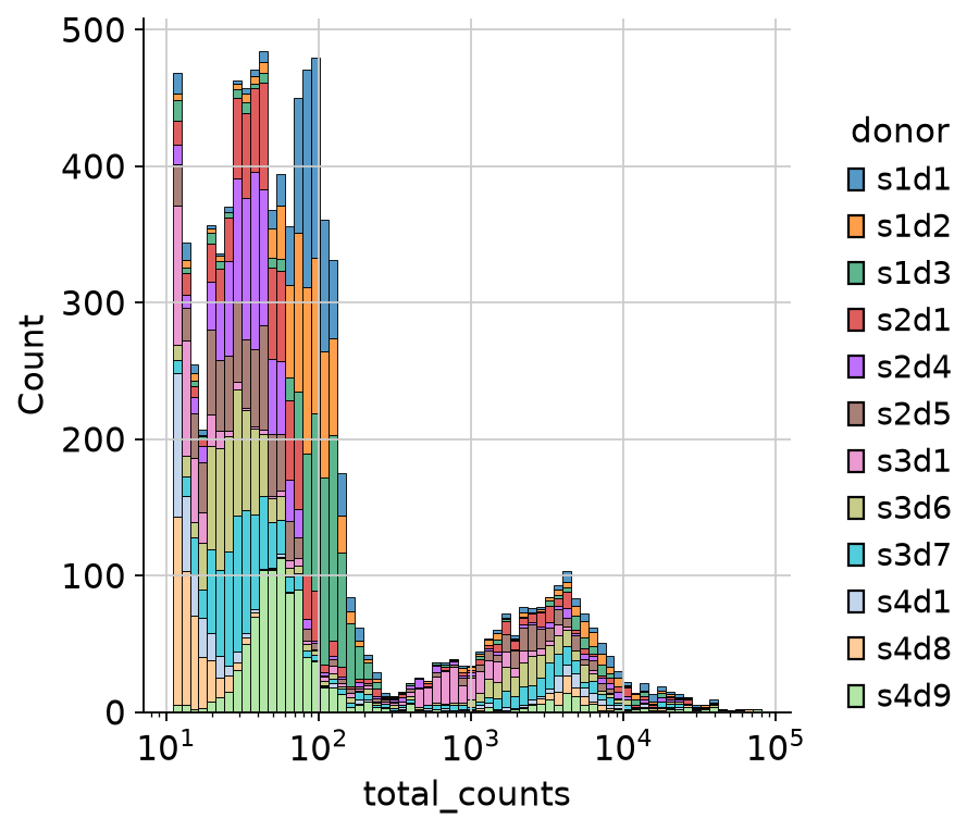

The first large peak between 10**1 and 10**2.1 is composed of droplets that don’t contain cells. We can use these cells for dsb normalization. In this case, the pre-processing software (often CellRanger) already differentiated droplets that contain cells and sorted them into the filtered data, here represented by the “mdata” object. Instead, the unfiltered data, here represented by the “mdata_raw” object, contains all droplets, both with and without cells. dsb normalization will use droplets without cells in order to estimate ambient noise and then remove it.

Additionally, we also now explicitly list the isotype controls that dsb normalization will use to remove noise from unspecific binding.

isotype_controls = ["Mouse-IgG1", "Mouse-IgG2a", "Mouse-IgG2b", "Rat-IgG2b"]

We now call the normalization function muon.prot.pp.dsb with the filtered and raw mudata object as well as the names of the isotype controls.

mu.prot.pp.dsb(mdata, mdata_raw, isotype_controls=isotype_controls, random_state=0)

Let’s have a look at counts before denoising and normalization.

pd.Series(mdata["prot"].layers["counts"][:100, :100].toarray().flatten()).value_counts()

1.0      1048
0.0      1026
2.0       898
3.0       688
4.0       581
         ... 
347.0       1
390.0       1
344.0       1
565.0       1
621.0       1
Name: count, Length: 543, dtype: int64

See how after denoising and normalization the range changed.

pd.Series(mdata["prot"].X[:100, :100].flatten()).value_counts()

8.529189     2
1.581845     1
8.613171     1
14.779234    1
7.079424     1
            ..
8.519451     1
2.257648     1
7.581913     1
40.300850    1
6.755094     1
Name: count, Length: 9999, dtype: int64

Now let’s take a look at how total protein counts of each cell changed before and after dsb normalization:

sns.histplot(mdata["prot"].layers["counts"].sum(axis=1), bins=50)
plt.title("Total counts per cell (raw)")
plt.xlim(0, 20000)

(0.0, 20000.0)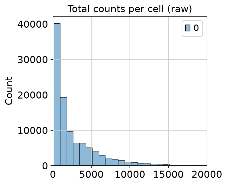

Before normalization, many cells have quite low total protein counts, while some cells have very high total protein counts. These very large differences in total protein counts are largely driven by ambient noise and unspecific binding.

sns.histplot(mdata["prot"].X.sum(axis=1), bins=50)
plt.title("Total counts per cell (dsb normalized)")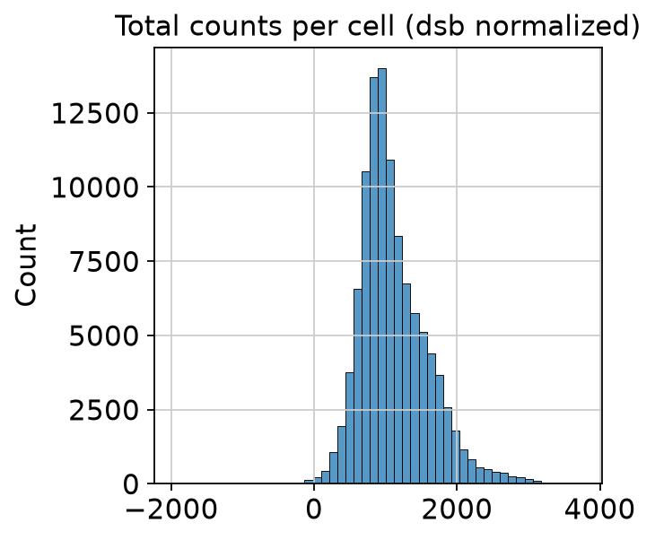

After normalization, the differences in total protein counts are much smaller and (probably) biology-driven rather than noise-driven.

Centered Log-Ratio normalization¶

If you don’t have the unfiltered data and/or the isotype controls available, you can also normalize the ADT data with muon.prot.pp.clr, implementing Centered Log-Ratio normalization. CLR normalization is the traditional way of normalizing ADT data, suggested in the original CITE-seq publication Stoeckius et al., 2017.

CLR normalization accounts for differences in sequencing depth (also called total counts) across cells, which can otherwise dominate downstream analyses. Cells with higher total ADT counts may appear artificially distinct, causing biologically similar cells to separate during clustering only based on their total ADT counts. CLR normalization rescales protein expression within each cell, making total ADT counts more similar in all cells. Specifically, it divides each protein count by the geometric mean of all protein counts in that cell and applies a log transformation.

mdata_clr_normalize = mdata.copy()
mdata_clr_normalize["prot"].X = mdata_clr_normalize["prot"].layers["counts"].copy()

Now we apply CLR normalization by using the function muon.prot.pp.clr:

mu.prot.pp.clr(mdata_clr_normalize["prot"], axis=1)

We recommend performing CLR normalization with axis=1, that is, normalizing each cell across proteins. This approach makes the total ADT counts more similar between cells, which is generally desirable for downstream analyses. The alternative is to perform CLR normalization with axis=0, normalizing each protein across cells. This makes the total ADT counts more similar between proteins, which is not generally desirable because proteins naturally exhibit substantial differences in abundance. An exception is experiments using only a small panel of antibodies that are expected to have similar overall count distributions, in which case axis=0 may be appropriate. Therefore, we recommend using axis=1 for most applications.

From muon version 0.1.8 onwards, there is a “flavor” argument. We currently use the default flavor=“seurat”, but note that flavor=“stoeckius” is another valid option.

We now compare the counts before and after normalization:

pd.Series(mdata["prot"].layers["counts"][:100, :100].toarray().flatten()).value_counts()

1.0      1048
0.0      1026
2.0       898
3.0       688
4.0       581
         ... 
347.0       1
390.0       1
344.0       1
565.0       1
621.0       1
Name: count, Length: 543, dtype: int64

pd.Series(mdata_clr_normalize["prot"].X[:100, :100].toarray().flatten()).value_counts()

0.000000    1026
0.172764      20
0.163880      19
0.160785      18
0.166124      17
            ... 
2.751836       1
1.074037       1
1.052570       1
1.923326       1
4.267047       1
Name: count, Length: 4092, dtype: int64

And we plot the distribution of total protein counts per cell:

sns.histplot(mdata_clr_normalize["prot"].X.sum(axis=1), bins=50)
plt.title("Total counts per cell (CLR normalized)")
plt.xlim(0, 400)

(0.0, 400.0)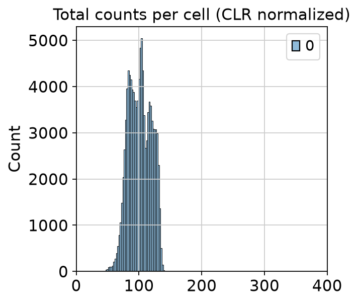

CLR normalization successfully reduced the difference in total protein counts. The range of total protein counts goes from 50 to 150, which is reasonable. If we compare this range with the range of differences in total protein counts in the raw data, which went from 0 to 20000, CLR normalization alleviated some of those differences, which were largely driven by experimental noise.

We save our dsb-normalized CITE-seq data, since dsb normalization is our method of choice when isotype controls and empty droplet data is available.

af_normalization = ln.Artifact.from_mudata(
    mdata,
    key="surface-protein/cite_normalization.h5mu",
    description="CITE-seq data after normalization",
)
af_normalization.save()

→ returning artifact with same hash: Artifact(uid='1gDVbNOjKn0egsqm0003', key='surface-protein/cite_normalization.h5mu', description='CITE-seq data after normalization', suffix='.h5mu', kind='dataset', otype='MuData', size=1467018249, hash='PntBph8LObdvBIRlb7XKEm', n_files=None, n_observations=106515, branch_id=1, created_on_id=1, space_id=1, storage_id=1, run_id=98, schema_id=None, created_by_id=7, created_at=2026-07-29 10:21:13 UTC, is_locked=False, version_tag=None, is_latest=True); to track this artifact as an input, use: ln.Artifact.get()

Artifact(uid='1gDVbNOjKn0egsqm0003', key='surface-protein/cite_normalization.h5mu', description='CITE-seq data after normalization', suffix='.h5mu', kind='dataset', otype='MuData', size=1467018249, hash='PntBph8LObdvBIRlb7XKEm', n_files=None, n_observations=106515, branch_id=1, created_on_id=1, space_id=1, storage_id=1, run_id=98, schema_id=None, created_by_id=7, created_at=2026-07-29 10:21:13 UTC, is_locked=False, version_tag=None, is_latest=True)

ln.finish()

• please hit CTRL + s to save the notebook in your editor ... ✓
→ finished Run('kGh9gDK6yaGvesDT') after 15m at 2026-07-29 10:54:55 UTC
→ go to: https://lamin.ai/theislab/sc-best-practices/transform/Z95qTilYUzGh0005
→ to update your notebook from the CLI, run: lamin save /groups/nils/members/javier/single-cell-best-practices/jupyter-book/surface_protein/normalization.ipynb

Contributors¶

We gratefully acknowledge the contributions of:

Authors¶

Javier Marchena-Hurtado
Daniel Strobl
Ciro Ramírez-Suástegui

Reviewers¶

Lukas Heumos
Anna Schaar

References¶

Zheng, Y., Jun, S.-H., Tian, Y., Florian, M., & Gottardo, R. (2022). Robust Normalization and Integration of Single-cell Protein Expression across CITE-seq Datasets. bioRxiv. 10.1101/2022.04.29.489989
Stoeckius, M., Hafemeister, C., Stephenson, W., Houck-Loomis, B., Chattopadhyay, P. K., Swerdlow, H., Satija, R., & Smibert, P. (2017). Simultaneous epitope and transcriptome measurement in single cells. Nature Methods, 14(9), 865–868. 10.1038/nmeth.4380
Mulè, M. P., Martins, A. J., & Tsang, J. S. (2022). Normalizing and denoising protein expression data from droplet-based single cell profiling. Nature Communications, 13(11), 2099. 10.1038/s41467-022-29356-8