Annotation - Single-cell best practices

Steps

yml

Install conda:
- Before creating the environment, ensure that conda is installed on your system.
Save the yml content:
- Copy the content from the yml tab into a file named environment.yml.
Create the environment:
- Open a terminal or command prompt.
- Run the following command:
```
conda env create -f environment.yml
```
Activate the environment:
- After the environment is created, activate it using:
```
conda activate <environment_name>
```
- Replace <environment_name> with the name specified in the environment.yml file. In the yml file it will look like this:
```
name: <environment_name>
```
Verify the installation:
- Check that the environment was created successfully by running:
```
conda env list
```

surface_protein.yml

name: surface-protein
channels:
  - conda-forge
dependencies:
  - python=3.13
  - scanpy=1.12
  - muon=0.1.9
  - python-igraph=1.0.0
  - ipykernel=7.2.0
  - pip==26.0.1
  - pip:
      - lamindb==2.3.1
      - harmonypy==0.0.9
      - ipywidgets==8.1.8

This book uses lamindb to store, share, and load datasets and notebooks using the theislab/sc-best-practices instance. We acknowledge free hosting from Lamin Labs.

Install lamindb
- Install the lamindb Python package:
```
pip install lamindb
```
Optionally create a lamin account
- Sign up and log in following the instructions
Verify your setup
- Run the lamin connect command:
```
import lamindb as ln

ln.Artifact.connect("theislab/sc-best-practices").df()
```
You should now see up to 100 of the stored datasets.
Accessing datasets (Artifacts)
- Search for the datasets on the Artifacts page
- Load an Artifact and the corresponding object:
```
import lamindb as ln
af = ln.Artifact.connect("theislab/sc-best-practices").get(key="key_of_dataset", is_latest=True)
obj = af.load()
```
The object is now accessible in memory and is ready for analysis. Adapt the lamindb.Artifact.connect("theislab/sc-best-practices").get("SOMEIDXXXX") suffix to get respective versions.
Accessing notebooks (Transforms)
- Search for the notebook on the Transforms page
- Load the notebook:
```
lamin load <notebook url>
```
which will download the notebook to the current working directory. Analogously to Artifacts, you can adapt the suffix ID to get older versions.

Motivation¶

Similar to scRNA-seq data, it is possible to annotate the ADT data based on surface protein markers. This can be very beneficial for the annotation of immune cells, since they are difficult to annotate in the RNA space and they are well described by their surface proteins. scRNA-seq data can suffer from dropouts, that is, although a gene is expressed in a cell population, the gene is not detected in some cells due to limitations of the sequencing procedure. Instead, ADT data does not suffer so much from dropouts due to using antibodies to quantify surface proteins. Therefore individual surface proteins show a stronger signal in the ADT data than in the RNA data. For example, although sequenced immune cells usually include CD45 cells, the CD45 gene is not always highly expressed in the RNA data. This can be mitigated by annotating (additionally) on the ADT level.

The general annotation workflow makes use of the same functions as for RNA data and no ADT-specific functions are required.

Environment setup¶

import warnings

import scanpy as sc

warnings.filterwarnings("ignore")
sc.settings.verbosity = 0
sc.set_figure_params(
    dpi=80,
    facecolor="white",
    frameon=False,
)

import lamindb as ln

ln.track()

→ connected lamindb: theislab/sc-best-practices
→ loaded Transform('BnpvfJLWjHuE0009', key='annotation.ipynb'), re-started Run('4qV0TQMofb5Skmfz') at 2026-07-29 14:38:23 UTC
→ notebook imports: lamindb-core==2.3.1 muon==0.1.9 scanpy==1.12.3
• recommendation: to identify the notebook across renames, pass the uid: ln.track("BnpvfJLWjHuE")

Loading the data¶

We load the MuData object we saved at the end of the previous chapter, Batch correction:

af = ln.Artifact.connect("theislab/sc-best-practices").get(
    key="surface-protein/cite_batch_correction.h5mu", is_latest=True
)
mdata = af.load()
mdata

Manual annotation¶

First, we check the expression of CD45. CD45 is an important marker of immune cells, especially lymphocytes.
CD45 activates Lck, which in turn is required to phosphorylate the TCR complex Courtney et al., 2019. Therefore, CD45 should be broadly expressed in our dataset, and even more highly expressed in T cells, and should have lower expression in erythroid cells and, to a lesser extent, in myeloid cells.

sc.pl.umap(mdata["prot"], frameon=False, color="CD45", vmax=20)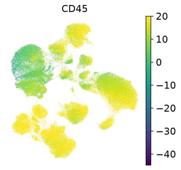

The measured ADTs use a slightly different nomenclature due to name clashes with RNA genes. The var_names_make_unique function was used to separate gene names from protein names and the proteins might have -1 suffixes. We look up an example gene name (CD38) to exemplarily find the exact nomenclature in our variable names:

mdata["prot"].var[mdata["prot"].var.gene_ids.str.contains("CD38")]

We cluster the cells with a relatively low resolution. Similarly to scRNA-seq data annotation, it is possible to increase the resolution for more fine-grained annotations.

sc.tl.leiden(
    mdata["prot"],
    resolution=0.08,
    flavor="igraph",
    n_iterations=2,
    directed=False,
    random_state=0,
)

To check which surface markers are differentially expressed in each cluster, we use the scanpy rank_genes_groups() function and then we create a dotplot. The dotplot will indicate the 3 most differentially expressed surface proteins in each cluster.

sc.tl.rank_genes_groups(mdata["prot"], groupby="leiden")
sc.tl.dendrogram(mdata["prot"], groupby="leiden")
sc.pl.rank_genes_groups_dotplot(
    mdata["prot"], n_genes=3, values_to_plot="logfoldchanges"
)

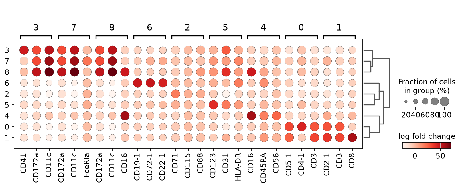
We can already identify clusters 0 and 1 as T cell populations by CD3 expression, and cluster 6 as B cells by CD19-1 expression. We next plot the UMAP that we calculated in our previous chapters and color it by cluster.

sc.pl.umap(mdata["prot"], color="leiden")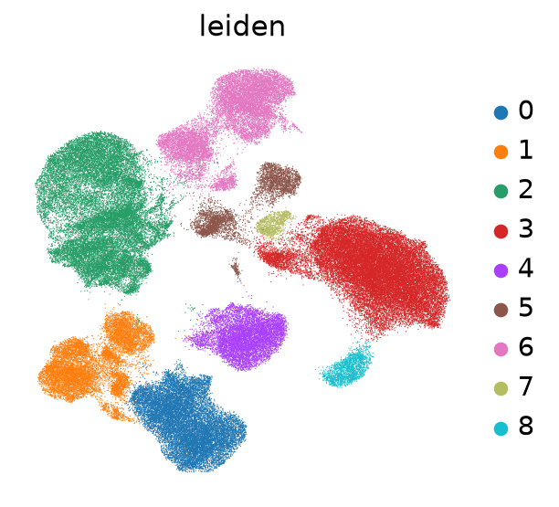

We’ll check a few known markers of major immune cell types in order to identify which cell type is each cluster.

# B cells
sc.pl.umap(mdata["prot"], frameon=False, color=["CD19-1"])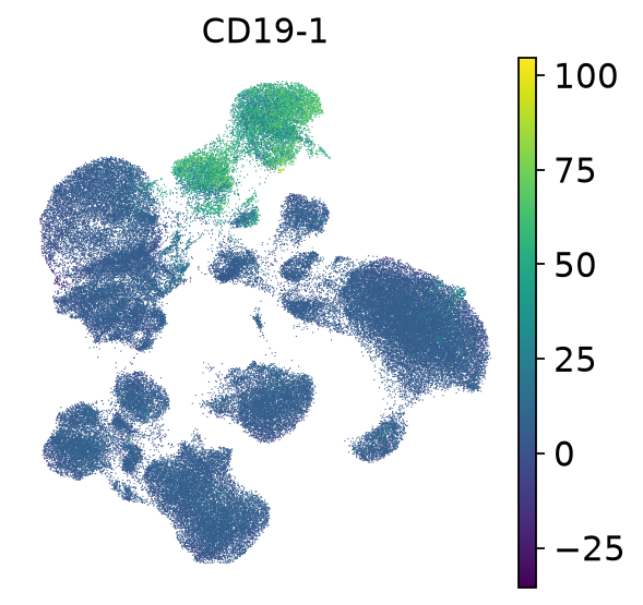

Cluster 6 expresses CD19 which is a B cell marker.

Let’s look into the T cells in more detail and separate them into CD4 and CD8 cells.

# T cells
sc.pl.umap(mdata["prot"], color=["CD3", "CD4-1", "CD8"])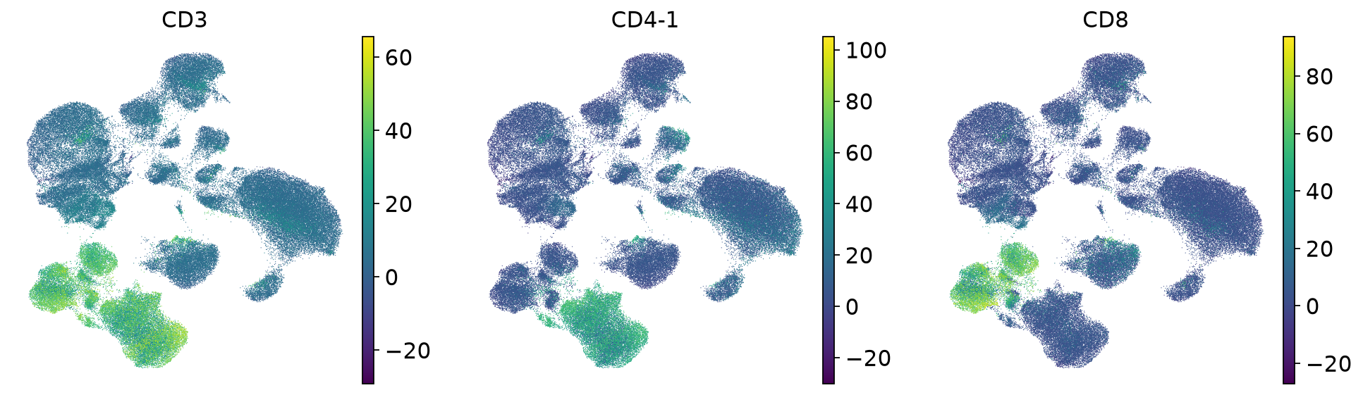

In the following few plots, we continue looking for known markers of other cell types: NK cells, CD14 monocytes, dendritic cells and CD16 monocytes.

# NK cells are CD3- and CD56+
# NKT cells are CD3+ and CD56+
sc.pl.umap(mdata["prot"], color=["CD56"], frameon=False)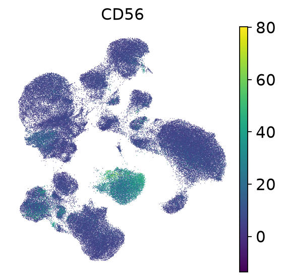

# CD14 Monocytes
sc.pl.umap(mdata["prot"], color=["CD11b", "CD14-1"], frameon=False, vmax=40)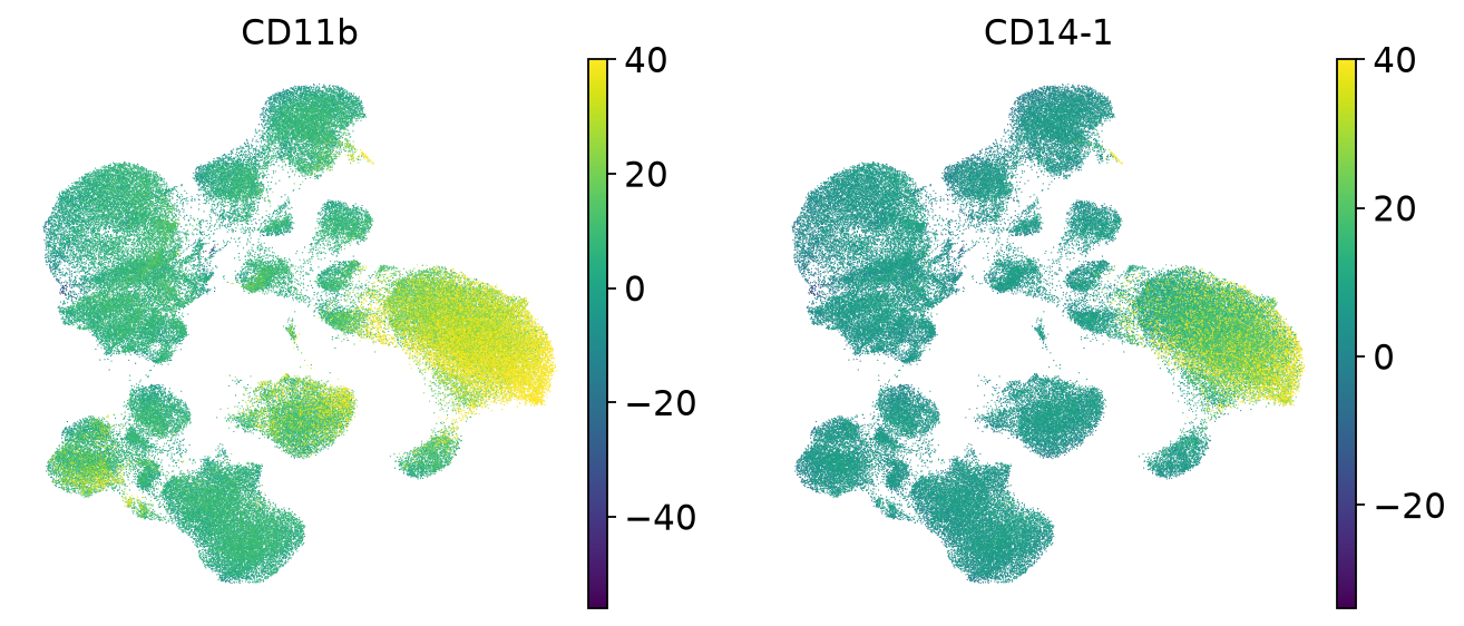

# Dendritic cells. CD123 and CD303 are expressed mostly in dendritic cells, while CD11c is expressed in myeloid cells, including dendritic cells.
sc.pl.umap(mdata["prot"], color=["CD123", "CD303", "CD11c"], frameon=False, vmax=30)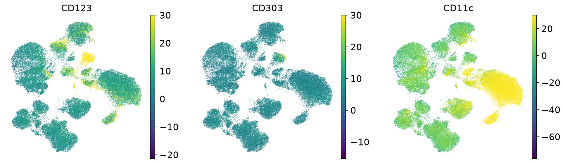

# CD16 is expressed in NK cells and in CD16 monocytes, which are CD14-, CD16+ and CD11c+
sc.pl.umap(mdata["prot"], color="CD16", frameon=False)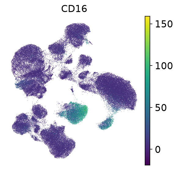

Now that we know what cell type each cluster is, let’s replace the 0-9 cluster numbers with the actual cell type names:

sc.pl.umap(mdata["prot"], color="leiden")

mdata["prot"].obs["celltype"] = mdata["prot"].obs.leiden.copy()
mdata["prot"].obs.celltype.replace(
    {
        "0": "CD4 T",
        "1": "CD8 T",
        "2": "Erythroid",
        "3": "CD14 Mono",
        "4": "NK",
        "5": "DC",
        "6": "B",
        "7": "DC",
        "8": "CD16 Mono",
    },
    inplace=True,
)

sc.pl.umap(
    mdata["prot"],
    color="celltype",
    legend_loc="on data",
    legend_fontsize=11,
    legend_fontoutline=2,
)

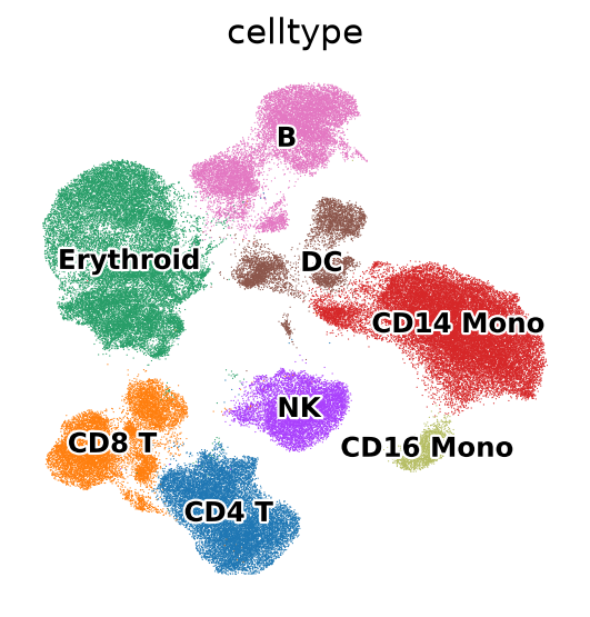
We have uncovered and annotated the main cell types in the data. Now we could perform a more fine-grained annotation by increasing the resolution of clustering and annotating the resulting fine-grained clusters.

In this chapter we describe how to annotate cell types based on the ADT data of CITE-seq. Another interesting way forward is to annotate cell types based on combined information from ADT and from RNA data. We refer to the Paired integration chapter for that.

af_annotation = ln.Artifact.from_mudata(
    mdata,
    key="surface-protein/cite_annotation.h5mu",
    description="CITE-seq data after annotation",
)
af_annotation.save()

→ creating new artifact version for key 'surface-protein/cite_annotation.h5mu' in storage 's3://lamin-eu-central-1/VPwcjx3CDAa2'
... uploading OyfKOZw9TXUQXeOp0006.h5mu: 100.0%
• replacing the existing cache path /var/cache/user/marchena/.cache/lamindb/lamin-eu-central-1/VPwcjx3CDAa2/surface-protein/cite_annotation.h5mu

Artifact(uid='OyfKOZw9TXUQXeOp0006', key='surface-protein/cite_annotation.h5mu', description='CITE-seq data after annotation', suffix='.h5mu', kind='dataset', otype='MuData', size=1450115558, hash='piMa8ZMc78O_eJtyyPlHCU', n_files=None, n_observations=105907, branch_id=1, created_on_id=1, space_id=1, storage_id=1, run_id=110, schema_id=None, created_by_id=7, created_at=2026-07-29 14:38:44 UTC, is_locked=False, version_tag=None, is_latest=True)

ln.finish()

• please hit CTRL + s to save the notebook in your editor ... ✓
→ finished Run('4qV0TQMofb5Skmfz') after 40s at 2026-07-29 14:39:03 UTC
→ go to: https://lamin.ai/theislab/sc-best-practices/transform/BnpvfJLWjHuE0009
→ to update your notebook from the CLI, run: lamin save /groups/nils/members/javier/single-cell-best-practices/jupyter-book/surface_protein/annotation.ipynb

Automated annotation¶

It is technically possible to use cell type classifiers trained on ADT data and to map against ADT reference datasets. However, ADT-specific methods are sparse if not non-existent, and we refer to the RNA annotation chapter for methodological details.

Contributors¶

We gratefully acknowledge the contributions of:

Authors¶

Javier Marchena-Hurtado
Daniel Strobl
Ciro Ramírez-Suástegui

Reviewers¶

Lukas Heumos
Anna Schaar

References¶

Courtney, A. H., Shvets, A. A., Lu, W., Griffante, G., Mollenauer, M., Horkova, V., Lo, W.-L., Yu, S., Stepanek, O., Chakraborty, A. K., & Weiss, A. (2019). CD45 functions as a signaling gatekeeper in T cells. Sci. Signal., 12(604), eaaw8151.