Bulk deconvolution

TL;DR We provide a brief overview over basic concepts of cell type deconvolution including input structure, data preprocessing and analysis of the output data.

Background¶

Studying differences in cell type compositions within a bulk tissue is important for several reasons. First, interactions between cell types play a major role in disease progression and recovery. Second, molecular patterns (such as gene expression and protein abundance) are often directly associated with the cell types compositions within the tissue. Understanding these compositions is crucial for studying the underlying molecular mechanisms of a biological condition such as disease. Third, uncovering disease-specific cell type patterns allow for better therapeutic targeting, providing an important clinical utility.

Cell type deconvolution is a computational framework designed for inferring the compositions of cell populations within a bulk heterogeneous tissue Kuhn et al., 2012Schwartz, 2010Du et al., 2019Zaitsev et al., 2019. As measuring these compositions experimentally is time-consuming and expensive, deconvolution methods allow large scale analysis of cell populations based on molecular data. Deconvolution methods usually follow linear regression defined as:

$y = bX$

where, $y$ refers to a mixture of heterogeneous gene expression profile using common molecular pipelines (e.g. microarray or RNA-seq), $X$ is a signature matrix containing homogeneous cell type-specific profiles, and $b$ is the vector of cellular proportions in the mixture data inferred by the deconvolution method Baron et al., 2016. To select an optimal deconvolution method suitable for the targeted biological conditions, the impact of several technical and biological factors should be considered including: the deconvolution method, reference data with missing or rare cell types, data normalization and the selection of features (markers).

The signature matrix $X$, used to infer cellular compositions, reflects our best knowledge of cellular heterogeneity within the tissue and highly influences the success of the deconvolution process Aliee & Theis, 2021. Originally, signature matrices were generated by profiling sorting cells from a heterogeneous tissue (using FACS or CyTOF), suffering from internal biases due to the pre-selection of cell type panels and the absence of appropriate antibodies Monaco et al., 2019Aran et al., 2017. Today, these matrices are mainly generated as unbiased profiles using single cell technologies, allowing the generation of signature matrices across different organisms, tissues and biological conditions Aliee & Theis, 2021Newman et al., 2019.

Approaches¶

Bulk deconvolution approaches can be divided into linear regression based methods, enrichment based methods, non-linear deep-learning based methods and others.

The most common type of cell type deconvolution methods are linear regression-based. These methods try to directly solve the $y = bX$ equation using different regularizations and relying on a relatively high number of features. Examples of such tools are CIBERSORTx Newman et al., 2019, MuSiC Wang et al., 2019, dtangle Hunt et al., 2018 and DWLS Tsoucas et al., 2019.

Enrichment based tools on the other hand calculate an enrichment score for each cell type separately, based on a gene set that represents this cell type. The enrichment scores for all cell types are then combined and transformed to compositions by a method-specific transformation function. As these methods only consider a single cell type at a time, tend to provide meaningful insights in simple cases, but are less accurate when reference data includes many cell types. xCell Aran et al., 2017 is an example of an enrichment based tool.

The third option pose non-linear deep learning methods that emerged with the promise of improving deconvolution accuracy, while still attempting to maintain high biological interpretability. It is still early to say whether these methods can be better than other types of methods. Scaden Menden et al., 2020 is an example of such a deep-learning based method.

Bulk deconvolution methods have been benchmarked extensively and the results are overall quite consistent Shen-Orr & Gaujoux, 2013Cobos et al., 2021Jin & Liu, 2021Nadel et al., 2021. Methods using single-cell RNA-seq data show good performance whereas semi-supervised approaches show higher error rates. Failing to include cell types in the reference that are present in the bulk mixture lead to worse results in any case Cobos et al., 2021. Cobos et al. recommend that (1) the input data should be in linear scale, (2) Avoid row scaling, column min-max, column z-score or quantile normalization, (3) regression bulk deconvolution methods like CIBERSORTx or FARDEEP Hao et al., 2019 perform well and if scRNA-seq data is available DWLS, MuSiC or SCDC Dong et al., 2020 should also be applied for result comparisons, (4) a stringent marker selection strategy that focuses on the differences between the first and second cell types with highest expression values should be used, (5) a comprehensive reference matrix that includes all relevant cell types that are present in the mixture should be used Cobos et al., 2021. The effect of the normalization strategy is unclear with Li et al. Li et al., 2016 suggesting that it has a strong effect on the results which was not confirmed by Cobos et al. Cobos et al., 2021.

Since many bulk deconvolution tools, including the well-performing CIBERSORTx, are only available as web tools, we opt to demonstrate a use-case with MuSiC.

It is important to note that MuSiC requires multiple single-cell samples including the same cell types. In practice, our reference profile might not include more than a single sample or some cell types might be missing across the samples. In these cases, MuSiC fails and another deconvolution method should be selected.

Deconvolving bulk COVID-19 whole blood samples¶

In the following use-case we deconvolve 49 bulk whole blood RNA-seq samples collected from 39 COVID-19 patients and 10 healthy controls Aschenbrenner et al., 2020 using MuSiC. As single-cell reference dataset we’ll use whole blood single-cell RNA-seq data of patients with COVID-19 Schulte-Schrepping et al., 2020.

Environment setup¶

Loading Data¶

We start by reading the single-cell and bulk data. We do not scale the data as it has been shown that deconvolution methods using scRNA-seq data as reference, perform best when applied to data in linear scale with improved accuracy after library size normalization Jin & Liu, 2021Cobos et al., 2021.

Data preprocessing¶

After reading the data, we need to remove undefined cells from our single-cell reference data. Here, we remove mixed and proliferating cells which are not limited to a single cell type.

Note Quality control by means of removing low quality cells and genes has already been performed on the single-cell data. So, we skip that.

It has been shown that deconvolution methods commonly fail to predict the proportion of rare cells Tsoucas et al., 2019. In case that you want to remove rare cell types, you can limit cell types to be above cellTypeNumCutOff cells. This cutoff is user-defined and should be selected based on the data.

We need to filter for the shared genes across bulk and single-cell data before selecting highly variable genes.

Visualization of single-cell data¶

For visualization of single-cell data, we first normalize the counts, select highly-variable genes and log transform the data.

We then reduce the dimensionality using PCA and visualize the data using UMAP:

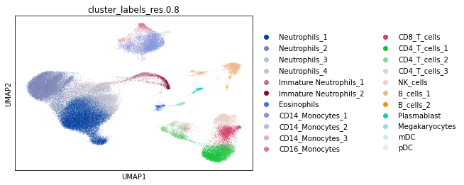
Deconvolving using MuSiC¶

Loading R¶

To use the R scripts, we need to convert the data from Python to R. In some cases, this requires sub-sampling of the data to avoid memory limitations.

If sub-sampling is not required (data is relatively small), one can simply convert the entire AnnData to an R object

Running MuSiC¶

We will first gather all the remaining inputs needed for running MuSiC:
1. adata_r - contains the single cell matrix which will used as a reference.
2. cell_subsets_r - cell type identities.
3. bulk - the bulk samples which the deconvolution process will be conducted on.
4. sc_genes - gene markers used in the MuSiC analysis.

MuSiC runs the deconvolution framework one sample at a time. Here, 9*** are sample names.

Outputs and Validations¶

The main output of all cell type deconvolution methods is a NxM matrix, where:
N (rows) - number of samples
M (columns) - the number of cell types
The values of each cell in the matrix represents the cell type composition of a specific cell type within a specific sample. In most cases, cell type compositions in a sample with be shown as fractions therefore, non-negative values, summing to one.

In case we know the true fractions of the cell types across sample, we can validate our deconvolved compositions. Here, Neutrophil counts were measured and indeed we found high correlations between the measured values and our deconvolution-based results.

We can also look for significant changes in cell compositions between disease patients and healthy controls. In this case, for each cell type, we calculate the p-value of this change based on student’s t-test.

Here is a boxplot presenting the differences between the two conditions

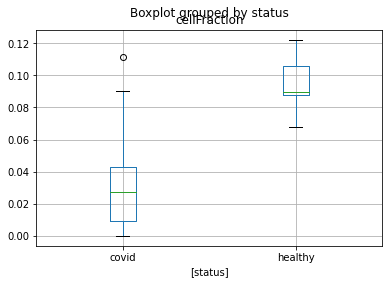
Limitations and traps¶

While single cell data is less prone to contain missing cell types, compared to pre-selected sorted cells, dealing with missing cell types is still considered a major challenge in the field of cell type deconvolution to this day Cobos et al., 2021Jin & Liu, 2021. In addition, the number of cell types within the signature matrix has a major influence on deconvolution accuracy, as more cell types usually results in a less accurate deconvolution process Newman et al., 2019.

While several deconvolution methods can correctly infer the proportion of major cellular components, their performance for rare or correlated components varies. To deal with the co-linearity between the predictors some methods perform feature selection prior deconvolution by selecting a subset of genes (called signature gene list) that minimizes the correlation between cell types.

New directions¶

Other than the methods we described before, there are additional tools which can be utilized to either improve deconvolution or deconvolve higher resolution states within cell types:

AutoGeneS Aliee & Theis, 2021 proposes a multi-objective feature selection method that can be integrated into a deconvolution platform. AutoGeneS requires no prior knowledge about marker genes and selects genes by simultaneously optimizing multiple criteria: minimizing the correlation and maximizing the distance between cell types. AutoGeneS can be applied to reference profiles from various sources like single-cell experiments or sorted cell populations.

CPM Frishberg et al., 2019 is a cell-state deconvolution method which allows discovering compositional changes occurring within each cell type, based on the single cell cell space, often capturing transitions in cell compositions across continuous cellular trajectories. By focusing on the variation within cell types, and less between cell types (as most deconvolution methods), CPM can discover changes in compositions of distinct subgroups of cells or continuous changes across specific cellular trajectories.

Contributors¶

We gratefully acknowledge the contributions of:

Authors¶

• Hananeh Aliee

• Amit Frishberg