🧠 Key takeaways
When applying Augur ensure that the cell types can be confidently labeled. Use differential abundance tests to find confounding effects and differential gene expression to find gene-level sources of perturbation effects.
Predicting perturbation responses with tools such as scGen works well for highly expressed genes, but is challenging for lowly expressed genes.
The linear discriminant analysis step of the Mixscape pipeline primarily aids with visualization. Distances in UMAPs should be interpreted with caution and therefore similarities and differences between knockouts cannot always be inferred at a glance.
⚙️ Environment setup
Install conda:
Before creating the environment, ensure that conda is installed on your system.
Save the yml content:
Copy the content from the yml tab into a file named
environment.yml.
Create the environment:
Open a terminal or command prompt.
Run the following command:
conda env create -f environment.yml
Activate the environment:
After the environment is created, activate it using:
conda activate <environment_name>Replace
<environment_name>with the name specified in theenvironment.ymlfile. In the yml file it will look like this:name: <environment_name>
Verify the installation:
Check that the environment was created successfully by running:
conda env list
name: perturbation_modeling
channels:
  - defaults
  - conda-forge
dependencies:
  - conda-forge::python=3.13.11
  - conda-forge::pertpy=1.0.4
Motivation
Advances in single-cell experimental protocols allow for massively multiplexed experiments to measure hundreds of thousands of cells under thousands of unique conditions. These are commonly termed “perturbations”, which are temporary or permanent changes caused by an external influence Srivatsan et al., 2020. Recently, such technologies have been adapted to profile CRISPR-Cas9 with multimodal readouts Papalexi et al., 2021Frangieh et al., 2021, genome-wide perturbations Replogle et al., 2021, and combinatorial perturbations Wessels et al., 2022. Despite experimental advances, exploring the massive perturbation space of combinatorial gene knock-outs or drug combinations remains challenging. The vast exploration space motivated the development of computational approaches for modeling single-cell perturbation responses Ji et al., 2021.
Perturbation modeling entails areasJi et al., 2021:
Perturbation responses: Predicting omics signatures after a perturbation given information about the control and treatment conditions. Predictions can be evaluated by the correlation of predicted features with respect to the true values. It is further possible to predict phenotypic measurements such as IC50 values, area under the dose response curve, toxicity and viability.
Targets and mechanisms: Predicting targets and mechanisms of perturbation using omics measurements. Drug mode of actions can be identified with perturbation modeling even for uncharacterized compounds.
Perturbation interactions: Predicting combinatorial effects of perturbations to gain an understanding of interlinked effects between genetics and drugs or combinations of drugs.
Chemical properties: Predicting chemical properties of perturbations using omics measurements such as molecular fingerprints, R groups, pharmacophores or even complete compounds.
Robust and accessible tooling for all of these steps is still under development. Hence, we will solely introduce three approaches for a subset of these tasks that can be tackled with single-cell perturbation data in the following sections:
Finding the cell types that were most affected by perturbations using Augur applied to Kang 2018 Kang et al., 2018.
Predicting the transcriptional response of single cells to perturbations using scGen applied to Kang 2018 Kang et al., 2018.
Quantifying the sensitivity of genetic CRISPR perturbations using Mixscape applied to Papalexi 2021 Papalexi et al., 2021.
Identifying the cell types most affected by perturbations
Motivation
Perturbations rarely have the same effect on all cells. In particular, different cell types or cells in different states in their cell cycle can be affected to varying degrees. Here we will leverage Augur by Skinnider et al. Skinnider et al., 2021Squair et al., 2021, which provides one way of quantifying the degree of response, for this purpose.
Limitations of Augur
Since Augur determines the degree of perturbation responses, it requires distinct cell types. If cell type labeling is challenging due to ongoing continuous, smooth processes or trajectories of gene expression such as cell differentiation, Augur might not allow for fine-grained enough rankings. Constructing a clustering tree describing the relationships of different clusters, which were used for cell type annotation, and applying Augur to all possible clustering resolutions, could determine the most suitable resolution and therefore annotation for the perturbation of interest Squair et al., 2021.
Further, cell types mediating tissue- or organism-level responses to specific perturbations might themselves comprise subpopulations of responder and non-responder cells. The assignment of cells into responder and non-responder cells itself can be inaccurate because cells of a given cell type could fall along a continuous trajectory of perturbation response intensity. However, Augur does not decipher the individual cells’ perturbation responses and simply aggregates them as averages for the cell types Squair et al., 2021.
Some perturbation effects might originate primarily from a change in relative abundance of a particular cell type. The subsampling procedure in Augur, however, discards any information about the relative abundances. In fact, Augur samples equal numbers of cells from each condition prior to cross-validation. Any change in the abundance of a particular cell type could be accompanied by changes in the intrinsic transcriptional profile of that cell type. Strong perturbations could even lead to scenarios where specific cell types are depleted completely or suddenly arise only when perturbed. Hence, it is advisable to perform differential abundance tests for every cell type to help contextualize the Augur analysis results Squair et al., 2021.
Here, we will use a fast reimplementation of the original R implementation of Augur using the perturbation analysis toolbox pertpy. pertpy leverages the scverse ecosystem and is therefore fully compatible with AnnData in the Python ecosystem.
Predicting cell type prioritization for IFN-β stimulation
To demonstrate Augur, we will use the Kang dataset, which is a 10x droplet-based scRNA-seq peripheral blood mononuclear cell (PBMC) dataset from 8 Lupus patients before and after 6h-treatment with INF-β (16 samples in total)Kang et al., 2018.
Our goal here is to decipher which cell types were most affected by INF-β treatment.
First, we import pertpy and scanpy.
import warnings

warnings.filterwarnings("ignore")
warnings.simplefilter("ignore")

# This is required to catch warnings when the multiprocessing module is used
import os

os.environ["PYTHONWARNINGS"] = "ignore"
import pertpy as pt
import scanpy as scpertpy provides a convenient data loader to access the Kang dataset.
adata = pt.dt.kang_2018()We rename label to condition and the conditions themselves for improved readability.
adata.obs.rename({"label": "condition"}, axis=1, inplace=True)
adata.obs["condition"].replace({"ctrl": "control", "stim": "stimulated"}, inplace=True)This dataset contains PBMCs Kang et al., 2018 across seven different cell-types.
adata.obs.cell_type.value_counts()cell_type
CD4 T cells 11238
CD14+ Monocytes 5697
B cells 2651
NK cells 1716
CD8 T cells 1621
FCGR3A+ Monocytes 1089
Dendritic cells 529
Megakaryocytes 132
Name: count, dtype: int64We now create an Augur object using pertpy based on our estimator of interest to measure how predictable the perturbation labels for each cell type in the dataset are. The options for the estimator are random_forest_classifier or logistic_regression_classifier for categorical data and random_forest_regressor for numerical data. All estimators make use of a Params class to define further parameters. Here, we will use a random_forest_classifier which is generally a solid and fast choice and suits our categorical data.
ag_rfc = pt.tl.Augur("random_forest_classifier")Next, we need to load the AnnData object into a format that Augur is comfortable with. This can be easily done with the load function of our Augur object.
loaded_data = ag_rfc.load(adata, label_col="condition", cell_type_col="cell_type")
loaded_dataAnnData object with n_obs × n_vars = 24673 × 15706
obs: 'nCount_RNA', 'nFeature_RNA', 'tsne1', 'tsne2', 'label', 'cluster', 'cell_type', 'replicate', 'nCount_SCT', 'nFeature_SCT', 'integrated_snn_res.0.4', 'seurat_clusters', 'y_'
var: 'name'
obsm: 'X_pca', 'X_umap'This allows us to run Augur with the predict function. Generally, Augur can be run in two modes:
A feature selection based on the original Augur implementation (
select_variance_feature=True) that is also the default. This approach removes features with little cell-to-cell variation within that cell type. We refer to the Augur Nature Protocols paper for more detailsSquair et al., 2021. When this feature selection is chosen the results are very similar to the Augur implementation in R.A feature selection based on
scanpy.pp.highly_variable_genes. This feature selection reduces the number of genes that are taken into account for model training and might result in inflated Augur scores, because the highly variable genes are very useful to separate cell types. However, this mode is faster and recovers effects of perturbations on cell types very well. We recommend it for very large datasets with perturbations that are expected to have a strong effect on specific cell types.
Since we do not expect INF-β to have an exceptional effect on specific cell types, we run Augur with the original Augur feature selection. To further increase the resolution, we set the subsample_size to 20 (default: 50) which corresponds to the number of cells to randomly draw per cell type.
v_adata, v_results = ag_rfc.predict(
loaded_data, subsample_size=20, n_threads=4, select_variance_features=True, span=1
)
v_results["summary_metrics"]The result table contains several evaluation metrics for the fitted model. For the interpretation of the cell type prioritization of the IFN-β response, only the mean_augur_score is relevant, which corresponds to the mean_auc. The higher the value, the easier it is for the fitted model to discern between control and perturbed cell states. Hence, the perturbation effect was stronger for this cell type. Let’s visualize this effect.
lollipop = ag_rfc.plot_lollipop(v_results)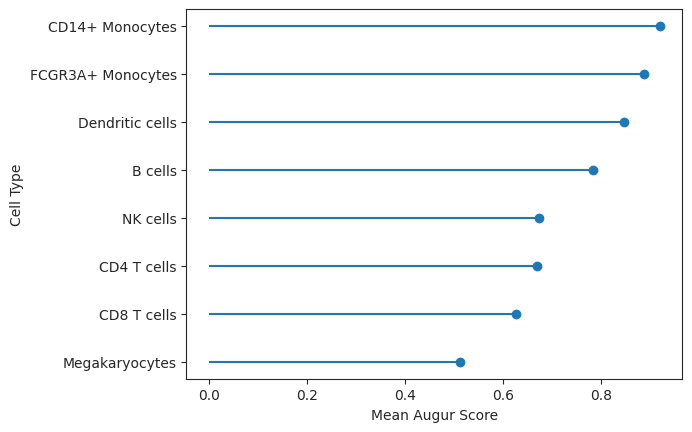
As observed, CD14+ Monocytes were the most affected by IFN-β whereas Megakaryocytes were the least affected. This corresponds roughly to the number of differentially expressed genes in the original publication for the respective cell types Kang et al., 2018.
The corresponding mean_augur_score is also saved in v_adata.obs and can be plotted in a UMAP.
sc.pp.neighbors(v_adata)
sc.tl.umap(v_adata)sc.pl.umap(adata=v_adata, color=["augur_score", "cell_type", "label"])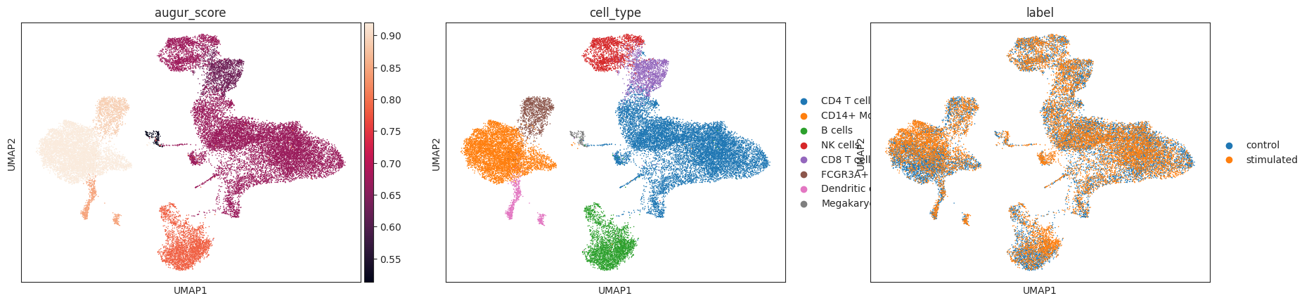
Determining the most important genes for the prioritization
The genes that contribute the most to the prioritization, as reflected by the augur score, correspond to the feature importances of our model. These feature importances are saved in the results object and can be easily plotted.
important_features = ag_rfc.plot_important_features(v_results)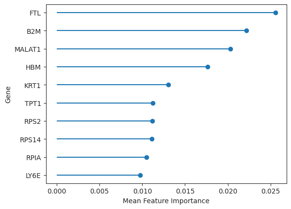
These genes could now be further explored concerning, for example, their role in pathways or other gene sets. However, since Augur performs inference on the cell type level, it does not directly determine the individual genes that are involved in the perturbation response. The authors of Augur themselves suggest using differential gene expression tests to be both conceptually and pragmatically a more appropriate approach to the inference at the level of individual genes Squair et al., 2021.
Differential prioritization
Augur is also able to perform differential prioritization by executing a permutation test to identify cell types with statistically significant differences in area under the curve (AUC) between two different rounds of cell type prioritization (for example a response to drugs A and B compared to untreated control).
Bhattacherjee et al. offered mice cocaine, and took samples of the prefrontal cortex for scRNA-seq at 48 hours and 15 days post withdrawalBhattacherjee et al., 2019.
We will now evaluate the effect of the withdraw_15d_Cocaine and withdraw_48h_Cocaine conditions compared to Maintenance_Cocaine. Basically, differential prioritization is obtained through a permutation test of the difference in AUC between two sets of cell-type prioritizations, compared with the expected AUC difference between the same two prioritizations after random permutation of sample labelsSquair et al., 2021. In this procedure, the user first performs cell-type prioritization on drug A (withdraw_15d_Cocaine) and drug B (withdraw_48h_Cocaine) separately, then calculates the AUC difference between drug A and drug B. To compute the statistical significance of the AUC difference , an empirical null distribution of AUC differences is then calculated for each cell type by permuting the sample labels, then repeating cell-type prioritization in the permuted data. Permutation P-values are then calculated. This procedure thus enables the identification of statistically significant differences in cell-type prioritization between conditions, as well as the condition in which the cell type is more transcriptionally separable.
Each variation is run once in default mode and once in permute mode to allow us to perform the permutation test. As a first step, we fetch the bhattacherjee dataset using pertpy and create an Augur object that again uses a random forest classifier.
bhattacherjee_adata = pt.dt.bhattacherjee()
ag_rfc = pt.tl.Augur("random_forest_classifier")Next, we run Augur on Maintenance_Cocaine and withdraw_15d_Cocaine using both augur_mode=default and augur_mode=permute as previously described. Note that we log normalize the dataset for a simple normalization.
sc.pp.log1p(bhattacherjee_adata)# Default mode
bhattacherjee_15 = ag_rfc.load(
bhattacherjee_adata,
condition_label="Maintenance_Cocaine",
treatment_label="withdraw_15d_Cocaine",
)
bhattacherjee_adata_15, bhattacherjee_results_15 = ag_rfc.predict(
bhattacherjee_15, random_state=None, n_threads=4
)
bhattacherjee_results_15["summary_metrics"].loc["mean_augur_score"].sort_values(
ascending=False
)Oligo 0.801417
Astro 0.769116
Microglia 0.743707
OPC 0.743605
Inhibitory 0.656202
NF Oligo 0.625692
Excitatory 0.623923
Endo 0.588481
Name: mean_augur_score, dtype: float64# Permute mode
bhattacherjee_adata_15_permute, bhattacherjee_results_15_permute = ag_rfc.predict(
bhattacherjee_15,
augur_mode="permute",
n_subsamples=100,
random_state=None,
n_threads=4,
)Now let’s do the same for Maintenance_Cocaine and withdraw_48h_Cocaine.
# Default mode
bhattacherjee_48 = ag_rfc.load(
bhattacherjee_adata,
condition_label="Maintenance_Cocaine",
treatment_label="withdraw_48h_Cocaine",
)
bhattacherjee_adata_48, bhattacherjee_results_48 = ag_rfc.predict(
bhattacherjee_48, random_state=None, n_threads=4
)
bhattacherjee_results_48["summary_metrics"].loc["mean_augur_score"].sort_values(
ascending=False
)Astro 0.624898
OPC 0.598050
NF Oligo 0.592619
Microglia 0.587789
Inhibitory 0.560000
Oligo 0.557630
Endo 0.540272
Excitatory 0.527143
Name: mean_augur_score, dtype: float64# Permute mode
bhattacherjee_adata_48_permute, bhattacherjee_results_48_permute = ag_rfc.predict(
bhattacherjee_48,
augur_mode="permute",
n_subsamples=100,
random_state=None,
n_threads=4,
)This allows us to take a look at the augur scores of the two runs in a scatterplot. The diagonal line is the identity function. If the values were the same they would be on the line.
scatter = ag_rfc.plot_scatterplot(bhattacherjee_results_15, bhattacherjee_results_48)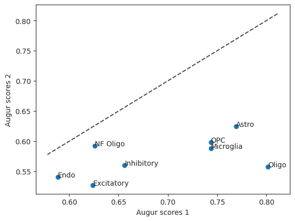
To figure out which cell type was most affected when comparing withdraw_48h_Cocaine and withdraw_15d_Cocaine we can run differential prioritization.
pvals = ag_rfc.predict_differential_prioritization(
augur_results1=bhattacherjee_results_15,
augur_results2=bhattacherjee_results_48,
permuted_results1=bhattacherjee_results_15_permute,
permuted_results2=bhattacherjee_results_48_permute,
)
pvalsThe p-value, following the R Augur implementation is calculated using b, the number of times permuted values are larger than original values and m, the number of permutations run. Since b is the same for all cells but Microglia, the p-value is the same for these as well.
diff = ag_rfc.plot_dp_scatter(pvals)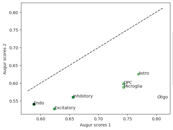
In this case the cell type “Inhibitory” is not very different between the two compared cell types which may indicate that permanent damage was inflicted.
Predicting IFN-β response for CD4-T cells
Many perturbation response modeling methods aim to forecast transcriptomic responses to stimuli, be it drugs, genetic knock-outs, or disease, for unseen populations where the perturbation response has not been measured, to help facilitate experimental design and hypothesis generation. The failure to capture cells treated with a perturbation could happen when a specific population could not be measured due to experimental or sample failure (e.g., failed cell sorting), high experimental costs prohibiting exploring all possibilities, and rare frequency of discovery for some cell types. In all scenarios above, an in-silico prediction of the missing population can lead to an informed decision about conducting new experiments or not.
Multiple methods for perturbation response modeling have been developed based on autoencoders (AE)Lotfollahi et al., 2019Lotfollahi et al., 2020Lotfollahi et al., 2021Russkikh et al., 2020Yuan et al., 2021Amodio et al., 2018Wei et al., 2022, a deep learning architecture to learn a low-dimensional representation of the data.
Here, we demonstrate the application of scGen Lotfollahi et al., 2019, a variational autoencoder combined with vector arithmetics. The model learns a latent representation of the data in which it estimates a difference vector between control (untreated) and perturbed (treated) cells. The estimated difference vector is then added to control cells for the cell type or population of interest to predict the gene expression response for each single cell. Here, we apply scGen to predict the response to IFN-β for a population of CD4-T cells that are artificially held out (unseen) during training to simulate one of the aforementioned real-world scenarios. We again leverage a dataset that contains peripheral blood mononuclear cells (PBMCs) from eight patients with Lupus treated with IFN-β or left untreated from Kang et al., 2018 across seven different cell-types.
As a first step, we import scanpy and scgen to allow us to work with AnnData objects and employ scGen.
import pertpy as pt
import scanpy as scSetting up the Kang dataset for scGen
We will again use pertpy to get the Kang dataset.
adata = pt.dt.kang_2018()scGen works best with log transformed data. Highly variable gene selection can speed up computations due to the reduced feature space.
sc.pp.log1p(adata)
sc.pp.highly_variable_genes(adata)We rename label to condition and the conditions themselves for improved readability.
adata.obs.rename({"label": "condition"}, axis=1, inplace=True)
adata.obs["condition"].replace({"ctrl": "control", "stim": "stimulated"}, inplace=True)
This dataset contains PBMCs Kang et al., 2018 across seven different cell-types.
adata.obs.cell_type.value_counts()cell_type
CD4 T cells 11238
CD14+ Monocytes 5697
B cells 2651
NK cells 1716
CD8 T cells 1621
FCGR3A+ Monocytes 1089
Dendritic cells 529
Megakaryocytes 132
Name: count, dtype: int64We remove all CD4T cells from the training data (adata_t) to simulate a real-world scenario of not capturing a specific population during an experiment.
adata_t = adata[
~(
(adata.obs["cell_type"] == "CD4 T cells")
& (adata.obs["condition"] == "stimulated")
)
].copy()
cd4t_stim = adata[
(
(adata.obs["cell_type"] == "CD4 T cells")
& (adata.obs["condition"] == "stimulated")
)
].copy()scGen requires the data to be in a particular format which is facilitated through AnnData and the setup_anndata function. It requires the key of the sample, the batch_key (in our case, "condition") and the cell type label key, the labels_key ("cell_type").
pt.tl.SCGEN.setup_anndata(adata_t, batch_key="condition", labels_key="cell_type")Model construction and training
scGen requires the modified AnnData object (adata_t) to construct the model object, which can be used to train the model. This function receives multiple user inputs, including the number of nodes in each hidden layer (n_hidden) of the model before the bottleneck layer (the middle layer of the network) and also the number of such layers (n_layers). Additionally, the user can adapt the dimension of the bottleneck layer, which is used to calculate the difference vector between perturbed cells and control cells. The default parameters used here are taken from the original publication. In practice, wider hidden layers lead to better reconstruction accuracy, which is essential for our aim to predict the perturbation response across many genes.
model = pt.tl.SCGEN(adata_t, n_hidden=800, n_latent=100, n_layers=2)scGen is a neural network with thousands of parameters to learn a low-dimensional data representation. Here, we use train method to estimate these parameters using the training data. There are multiple parameters here, max_epochs is the maximum number of iterations the model is allowed to update its parameters which are set to 100 here. The higher values training epochs will take more computation time but might help better results. The batch_size is the number of samples (individual cells) the model sees to update its parameters. Lower numbers usually lead to better results in the case of scGen. Finally, there is early_stopping, which enables the model to stop the training if its results are not improved after early_stopping_patience training epochs. The early stopping mechanism prevents potential overfitting of the training data, which can lead to poor generalization to unseen populations.
model.train(
max_epochs=100, batch_size=32, early_stopping=True, early_stopping_patience=25
)INFO Jax module moved to TFRT_CPU_0.Note: Pytorch lightning will show GPU is not being used for the Trainer.
GPU available: False, used: False
TPU available: False, using: 0 TPU cores
IPU available: False, using: 0 IPUs
HPU available: False, using: 0 HPUs
Epoch 26/100: 26%|██▌ | 26/100 [1:28:13<4:11:07, 203.61s/it, v_num=1, train_loss_step=1.06e+3, train_loss_epoch=4.52e+3]
Monitored metric elbo_validation did not improve in the last 25 records. Best score: 479.507. Signaling Trainer to stop.
To visualize the learned representation of data by the model, we plot the latent representation of the model using the UMAP algorithm. The get_latent_representation() returns a 100-dimensional vector for each cell. We store the latent representations in the .obsm slot of the AnnData object.
adata_t.obsm["scgen"] = model.get_latent_representation()Next, we recalculate the neighbors graph and the UMAP embedding using the calculated latent representation to finally visualize the new embedding in a UMAP plot.
sc.pp.neighbors(adata_t, use_rep="scgen")
sc.tl.umap(adata_t)sc.pl.umap(adata_t, color=["condition", "cell_type"], wspace=0.4, frameon=False)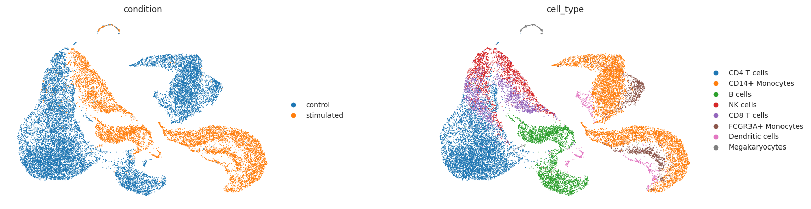
As observed above, the IFN-β stimulation induced strong transcriptional changes across all cell-types
Predicting CD4T responses to IFN-β stimulation
After the model is trained, we can ask the model to simulate the effect of IFN-β response for each control CD4T cell present in the training data. The prediction is made possible via the predict method, which receives the corresponding labels (ctrl_key and stim_key below) in the condition (as provided earlier by the user) column of the AnnData object to estimate a global difference vector in the latent space between ‘control’ and ‘stimulated’ cells. This vector is then added to each single-cell present specified in celltype_to_predict (here CD4T).
pred, delta = model.predict(
ctrl_key="control", stim_key="stimulated", celltype_to_predict="CD4 T cells"
)
# we annotate the predicted cells to distinguish them later from ground truth cells.
pred.obs["condition"] = "predicted stimulated"INFO Received view of anndata, making copy.
INFO Input AnnData not setup with scvi-tools. attempting to transfer AnnData setup
INFO Received view of anndata, making copy.
INFO Input AnnData not setup with scvi-tools. attempting to transfer AnnData setup
INFO Received view of anndata, making copy.
INFO Input AnnData not setup with scvi-tools. attempting to transfer AnnData setup
Evaluating the predicted IFN-β response
In previous sections, we predicted the response to IFN-β for each CD4T cell present among the control population. Since single-cell sequencing is destructive, meaning that cells can not be measured before and after a particular perturbation, it is impossible to directly evaluate the prediction for the same cell after IFN-β stimulation. However, we have a group of cells in the data treated with IFN-β, which we can use to measure how well the predicted cell population aligns with ground truth cells. To pursue this, we evaluate predictions qualitatively by looking at the embedding of control, predicted, and actual CD4T IFN-β cells in principal component analysis (PCA) space. Additionally, we also quantitatively measure the correlation between mean gene expression of predicted cells and IFN-β across all genes and differentially expressed genes after IFN-β stimulation.
First, we construct an AnnData object containing control, predicted stimulated, and actual stimulated cells.
ctrl_adata = adata[
((adata.obs["cell_type"] == "CD4 T cells") & (adata.obs["condition"] == "control"))
]
# concatenate pred, control and real CD4 T cells in to one object
eval_adata = ctrl_adata.concatenate(cd4t_stim, pred)eval_adata.obs.condition.value_counts()condition
stimulated 5678
control 5560
predicted stimulated 5560
Name: count, dtype: int64We first look at the PCA co-embedding of control, IFN-β stimulated and predicted CD4T cells.
sc.tl.pca(eval_adata)
sc.pl.pca(eval_adata, color="condition", frameon=False)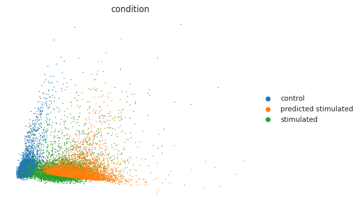
As observed above, the predicted stimulated cells were moved towards the CD4T stimulated cells with IFN-β. Yet we should also look at differentially expressed genes (DEGs) to verify whether the most striking DE genes are also present in the predicted stimulated cells. Below, we look at the overall mean correlation between predicted and real cells. Before that, we extract DEGs between control and stimulated cells:
cd4t_adata = adata[adata.obs["cell_type"] == "CD4 T cells"]We estimate DEGs using scanpy’s implementation of the Wilcoxon test.
sc.tl.rank_genes_groups(cd4t_adata, groupby="condition", method="wilcoxon")
diff_genes = cd4t_adata.uns["rank_genes_groups"]["names"]["stimulated"]
diff_genesarray(['ISG15', 'IFI6', 'ISG20', ..., 'EEF1A1', 'FTH1', 'RGCC'],
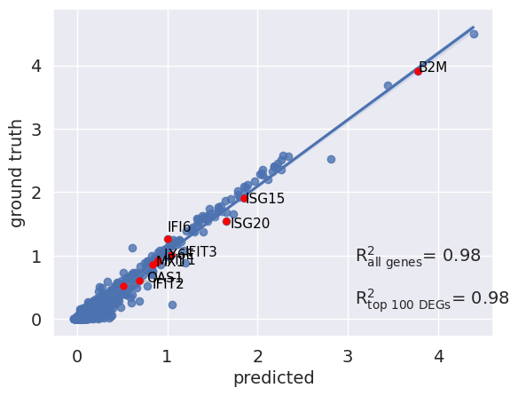
dtype=object)scGen features a reg_mean_plot that calculates the R² correlation between mean gene expression of predicted and existing IFN-β cells. The higher the R² (max is 1), the more faithful is the prediction compared to the ground truths. The highlighted genes in red are the top 10 upregulated DEGs after IFN-β stimulation, which are essential for a successful prediction. As observed, the model did a good job for genes with higher mean values, while it failed for some genes with a mean expression between 0-1. We also measure accuracy across non-DEGs because the model should not change genes not affected by the perturbation while changing the expression of DEGs.
r2_value = model.plot_reg_mean_plot(
eval_adata,
condition_key="condition",
axis_keys={"x": "predicted stimulated", "y": "stimulated"},
gene_list=diff_genes[:10],
top_100_genes=diff_genes,
labels={"x": "predicted", "y": "ground truth"},
show=True,
legend=False,
)
We can additionally look at the distribution of the top upregulated genes by IFN-β. For example, we plotted the distribution of expression in ISG15, a well-known gene induced after IFN stimulation. As observed, the model identified that this gene should be upregulated after stimulation with IFN-β, and it indeed shifted values to a similar range in ground-truth (stimulated) cells.
sc.pl.violin(eval_adata, keys="ISG15", groupby="condition")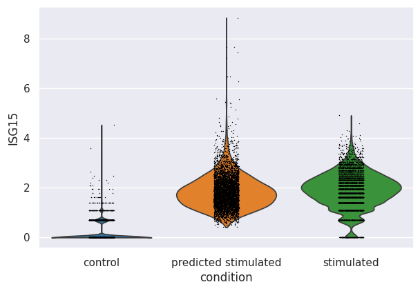
Overall, we demonstrated the application of scGen as an example of perturbation response models in predicting gene expression of the unseen population under desired perturbations. While perturbation response models provide in silico predictions, they cannot replace performing actual experiments. It is also unclear how much of the predicted response is attributed to cell type specific responses or across cell types. However, as observed in the case of scGen, it can predict the overall response for highly expressed genes yet provide poorer predictions for lowly expressed genes, which requires further optimization and motivation for developing more sophisticated and robust approaches.
Analysing single-pooled CRISPR screens
Expanded CRISPR-compatible CITE-seq (ECCITE-seq) enables the capture of single guide RNA (sgRNA) sequences together with transcriptome and surface protein measurements in the form of antibody-derived tags (ADTs). This allows for the application of many genetic perturbations together with transcriptomics readouts for effect exploration and validation of the perturbations through protein expression, making this assay very powerful. However, this power comes not only with great responsibility, but also with complexity.
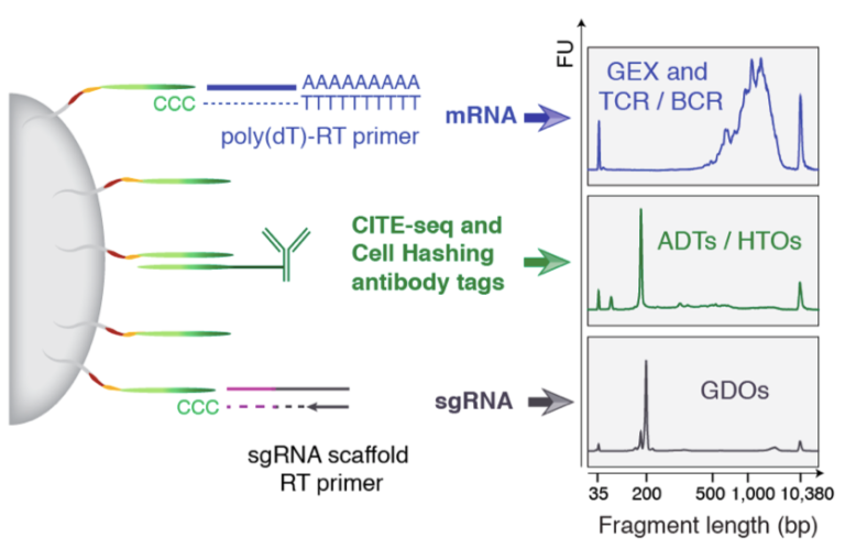
Figure 1:ECCITE-seq overview. mRNA is measured together with surface protein expression using antibody derived tags. Biological replicates are resolved through hashtag-derived oligonucleotides. The assignment of the guide RNAs is done using guide-derived oligonucleotides. Image obtained from (https://
For the purpose of this analysis we will be using the Papalexi 2021 dataset Papalexi et al., 2021. This dataset contains about 20000 stimulated THP-1 cells that used 111 gRNAs. THP-1 cells stimulated with a combination of IFN-y, decitabine (DAC) and transforming growth factor (TGF)-β1 results in an induction of three immune checkpoints: programmed death-ligand 1 (PD-L1), PD-L2 and CD86. The goal of the ECCITE-seq experiment was to investigate molecular networks that regulate PD-L1 expression, because it is frequently observed in human cancers and can suppress T-cell-mediated immune responses Papalexi et al., 2021.
For this specific analysis, we want to:
Remove confounding sources of variation such as cell cycle effects or batch effects.
Determine which cells were affected by the desired perturbations and which cells escaped.
Visualize perturbation responses.
To conduct this analysis we will again use pertpy which implements the Mixscape pipeline for the scverse ecosystem about 5-10x faster. This pipeline was originally developed for the Seurat ecosystem, and we largely follow the accompanying Seurat Vignette (https://
We start by importing pertpy, scanpy and muon, which we will require for the preprocessing of the protein data.
import muon as mu
import pertpy as pt
import scanpy as scAs a first step we fetch the dataset using pertpy. The return type of the dataloader is a MuData object containing the transcriptomics measurements, the ADT measurements and guide RNA counts.
mdata = pt.dt.papalexi_2021()
mdataThe original Seurat object contained four assays which were transformed into individual AnnData objects to then create the here downloaded MuData object. The individual modalities are:
adt: A count matrix of the four captured antibody-derived tags (CD86, PDL1, PDL2, CD366) which are also commonly simply referred to as “proteins” in this setting.gdo: The 111 used guide RNAs (gRNA). To assign a gRNA identity to each cell, guide-derived oligonucleotide (GDO) counts were examined. If a cell had less than five counts for all gRNA sequences, it was classified as negative. For all other cells, the gRNA with the highest number of counts was assigned to that cell. Cells that had high counts for more than one gRNA were classified as doublets.hto: To keep track of the identity of each biological replicate, the samples were hashed using hashtag-derived oligonucleotides (HTO) following the cell hashing protocol Stoeckius et al., 2018.rna: This corresponds to the transcriptome measurements for all cells and is the usual cells by genes count matrix.
Preprocessing
We keep the preprocessing of the RNA and ADTs simple. First, we normalize the RNA using scanpy’s normalize_total followed by log transformation and highly variable gene selection. To normalize the ADTs we apply centered log ration transformation Stoeckius et al., 2017.
sc.pp.normalize_total(mdata["rna"])
sc.pp.log1p(mdata["rna"])
sc.pp.highly_variable_genes(mdata["rna"], subset=True)mu.prot.pp.clr(mdata["adt"])Data exploration
To get a feeling for our dataset we visualize the replicates, cell-cycle phases and perturbations in a UMAP embedding.
sc.pp.pca(mdata["rna"])# We calculate neighbors with the cosine distance similarly to the original Seurat implementation
sc.pp.neighbors(mdata["rna"], metric="cosine")sc.tl.umap(mdata["rna"])sc.pl.umap(mdata["rna"], color=["replicate", "Phase", "perturbation"])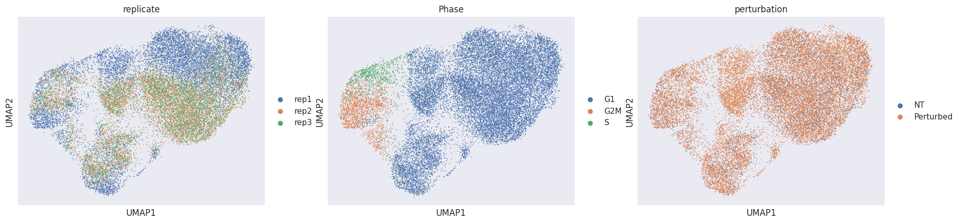
When glancing at the UMAPs we identify two clearly visible issues:
Many cells are separated by replicate ID. This is a common sign of a batch effect.
The cell cycle phase is a confounder in the embedding.
Hence, we now try to project our cells into a perturbation space by calculating local perturbation signatures to mitigate these identified issues.
Calculating local perturbation signatures
To alleviate the aforementioned issues, we will calculate local perturbation signatures. The core idea is that by subtracting the averaged expression of the k nearest cells from the control pool (=NT) from every cell, we retrieve the component of every cell that solely reflects the genetic perturbation. The k nearest neighbors must be in a biological state matching the target cell, but are not allowed to have been targeted by any gRNA. The obtained component is denoted as the local perturbation signature. By default, the number of neighbors k is set to 20. Following the recommendations of Papalexi et al., we recommend setting from the range of 20 < k 30. A k that is too small or too large is unlikely to remove any technical variation from the dataset Papalexi et al., 2021.
We now create a Mixscape object using pertpy and calculate the perturbation signature.
ms = pt.tl.Mixscape()

ms.perturbation_signature(
    mdata["rna"],
    pert_key="perturbation",
    control="NT",
    split_by="replicate",
    n_neighbors=20,
)
# We create a copy of the object to recalculate the PCA.
# Alternatively we could replace the X of the RNA part of our MuData object with the `X_pert` layer.
adata_pert = mdata["rna"].copy()
adata_pert.X = adata_pert.layers["X_pert"]
sc.pp.pca(adata_pert)
sc.pp.neighbors(adata_pert, metric="cosine")
sc.tl.umap(adata_pert)
sc.pl.umap(adata_pert, color=["replicate", "Phase", "perturbation"])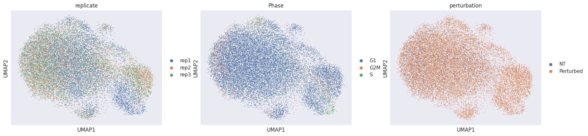
Using the perturbation signature to calculate the neighbors graph and the eventual embedding removes technical variation and reveals one additional perturbation-specific cluster. Now that our data is mostly free of confounding effects, we need to determine for which targeted cells (=perturbed) the perturbation was successful (=KO) or not (=NP).
Identifying cells with no detectable perturbation
The primary assumption that we make is that every target gene class is a mixture of two Gaussian distributions. One of these represents the successful knockouts (KO) and the other the non-perturbed (NP) cells. The distribution of the NP cells should then be identical to the cells expressing non-targeting gRNAs (NT). After having estimated the distribution of the KO cells, Mixscape calculates the posterior probability that a cell belongs to the KO distribution and classifies cells with a probability of more than 0.5 as KOs. Applying this to all 11 target gene classes allows us to identify all KO cells while evaluating the targeting efficacy of the different gRNAs.
ms.mixscape(adata=mdata["rna"], control="NT", labels="gene_target", layer="X_pert")We can now plot the class distributions for all 111 gRNAs.
ms.plot_barplot(mdata["rna"], guide_rna_column="guide_ID")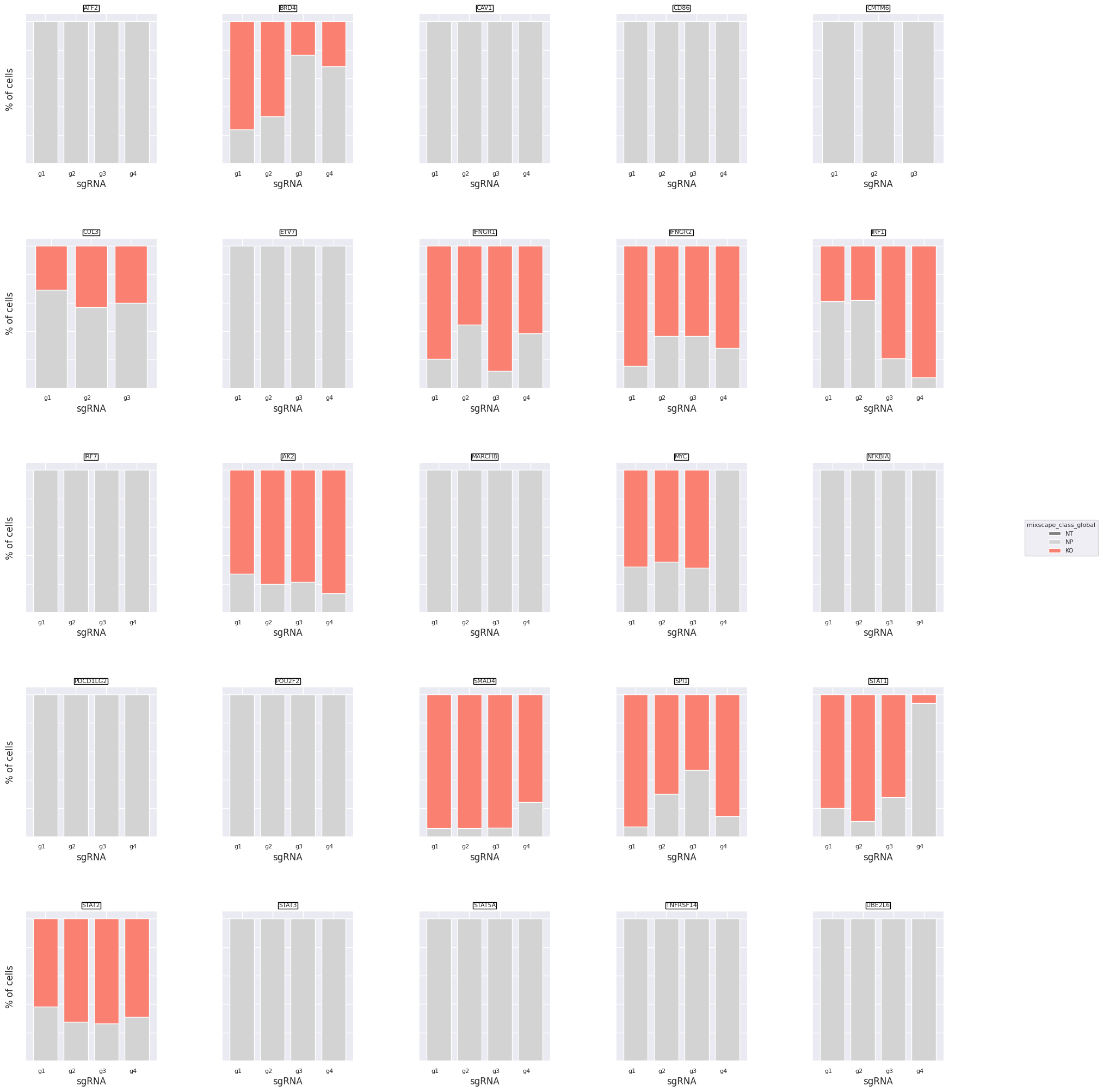
<Axes: title={'center': 'UBE2L6'}, xlabel='sgRNA', ylabel='% of cells'>We detect variation in gRNA targeting efficiency within each class. For example gRNA 4 for STAT1 did not seem to be very effective, but gRNA 1-3 were.
Let’s inspect the perturbation scores of an example target gene (IFNGR2).
ms.plot_perturbscore(
    adata=mdata["rna"], labels="gene_target", target_gene="IFNGR2", color="orange"
)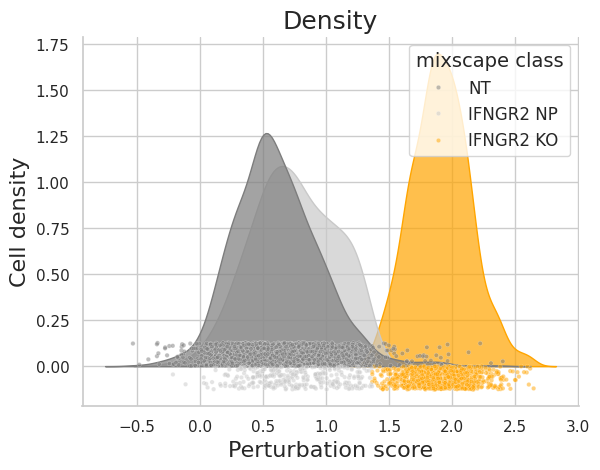
As expected, the distributions of the NT and IFNGR2 NP classes match rather well, whereas the IFGNR2 KO distribution is clearly shifted. This should also be reflected in the posterior probabilities.
sc.settings.set_figure_params(figsize=(10, 10))
ms.plot_violin(
    adata=mdata["rna"],
    target_gene_idents=["NT", "IFNGR2 NP", "IFNGR2 KO"],
    groupby="mixscape_class",
)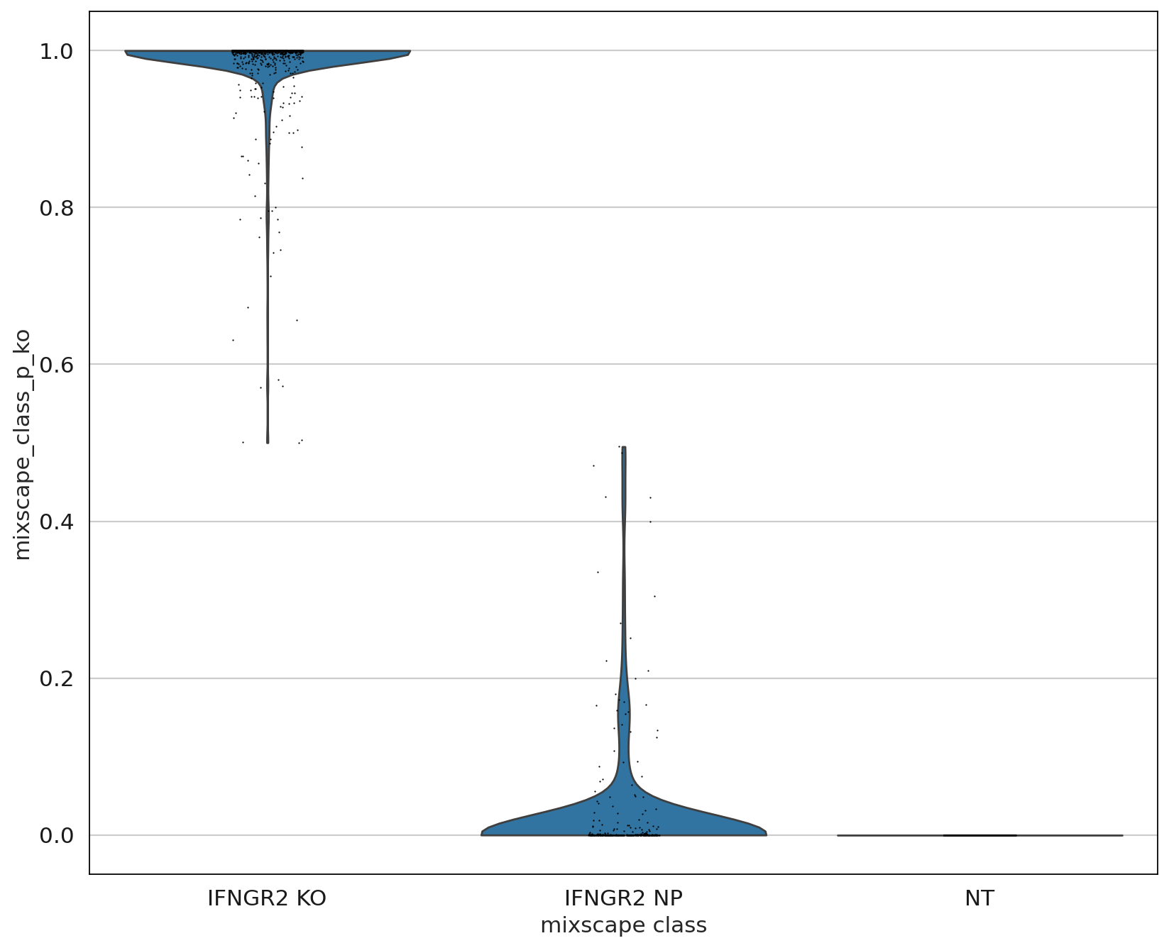
The posterior probabilities clearly separate the two classes highlighting very few unclear cases. This can be further highlighted by running a simple DE test between the mixscape classes and visualizing the results on a heatmap by ordering the posterior probabilities.
ms.plot_heatmap(
    adata=mdata["rna"],
    labels="gene_target",
    target_gene="IFNGR2",
    layer="X_pert",
    control="NT",
)
WARNING: dendrogram data not found (using key=dendrogram_mixscape_class). Running `sc.tl.dendrogram` with default parameters. For fine tuning it is recommended to run `sc.tl.dendrogram` independently.
WARNING: Groups are not reordered because the `groupby` categories and the `var_group_labels` are different.
categories: IFNGR2 KO, IFNGR2 NP, NT
var_group_labels: NT
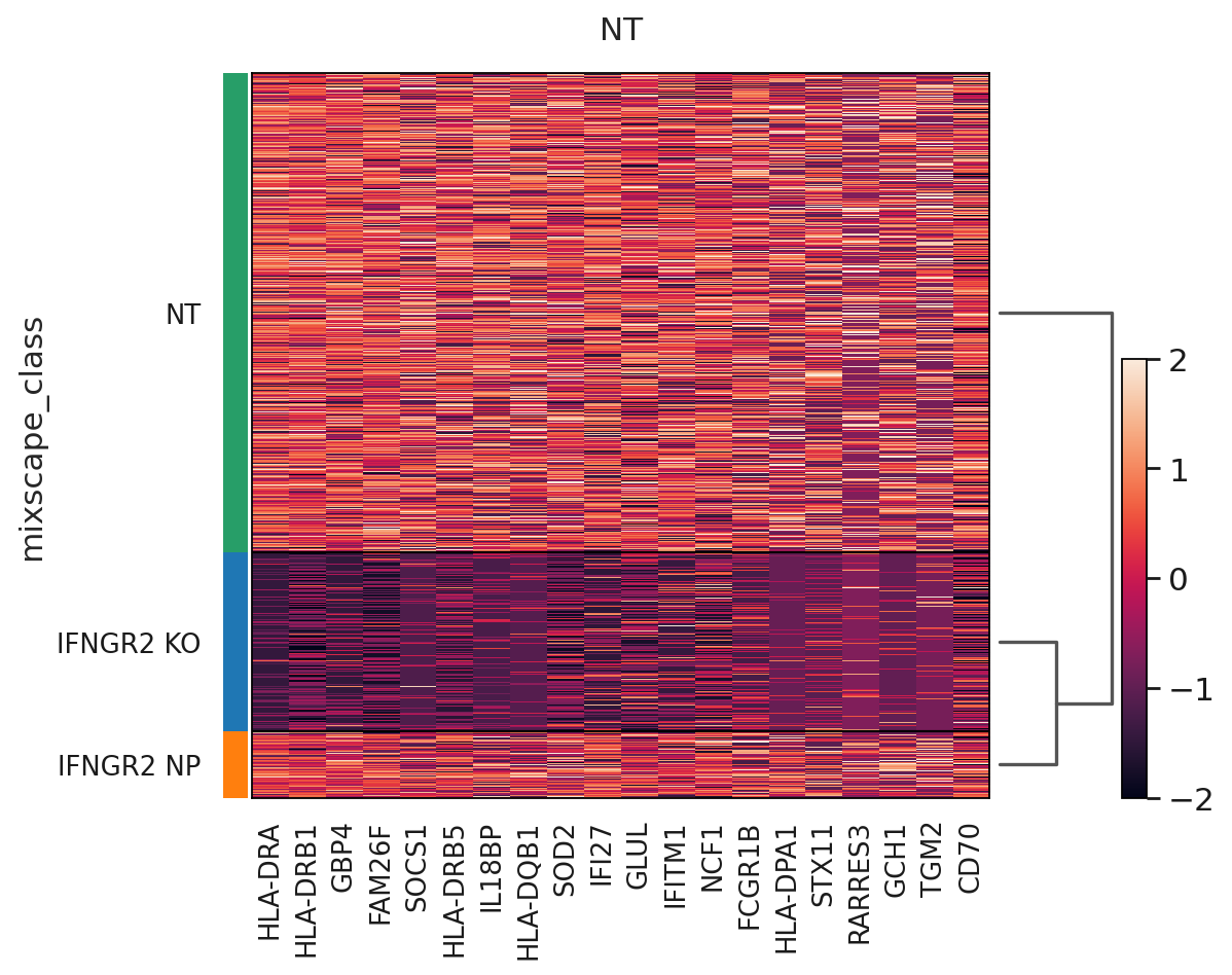
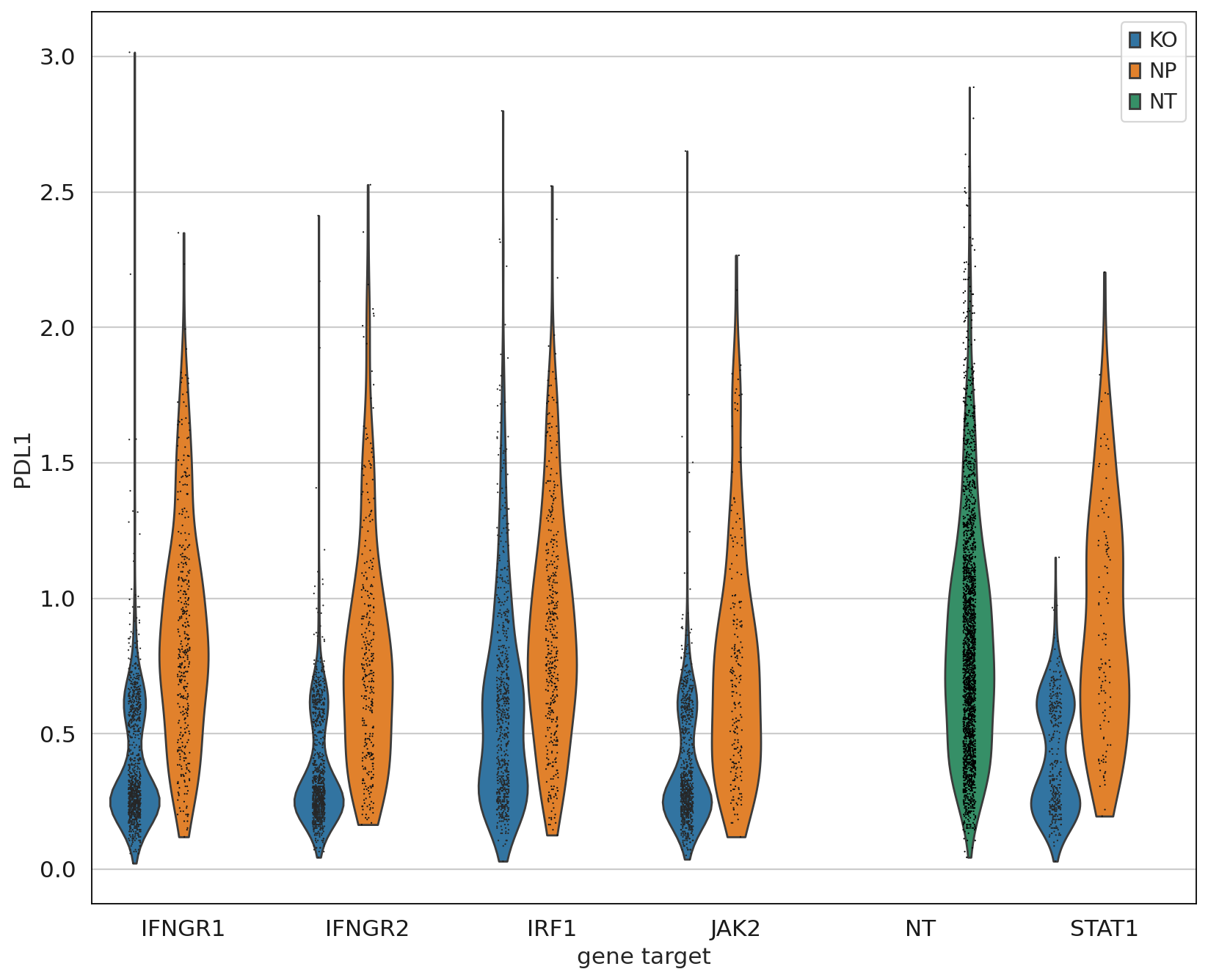
Up to this point we have only been working with the transcriptomics data, but we can now leverage the measured proteins to demonstrate that only IFGN pathway KO cells have a reduction in PDL1 expression.
mdata["adt"].obs["mixscape_class_global"] = mdata["rna"].obs["mixscape_class_global"]
ms.plot_violin(
    adata=mdata["adt"],
    target_gene_idents=["NT", "JAK2", "STAT1", "IFNGR1", "IFNGR2", "IRF1"],
    keys="PDL1",
    groupby="gene_target",
    hue="mixscape_class_global",
)
Visualizing perturbation responses with Linear Discriminant Analysis
The final step in the Mixscape pipeline is to calculate and visualize perturbation-specific clusters. This is done by applying linear discriminant analysis (LDA) and recalculating the UMAP using the determined results. LDA attempts to maximize the separability of known labels, which are the mixscape classes in our case, using both gene expression and the labels.
ms.lda(adata=mdata["rna"], control="NT", labels="gene_target", layer="X_pert")ms.plot_lda(adata=mdata["rna"], control="NT")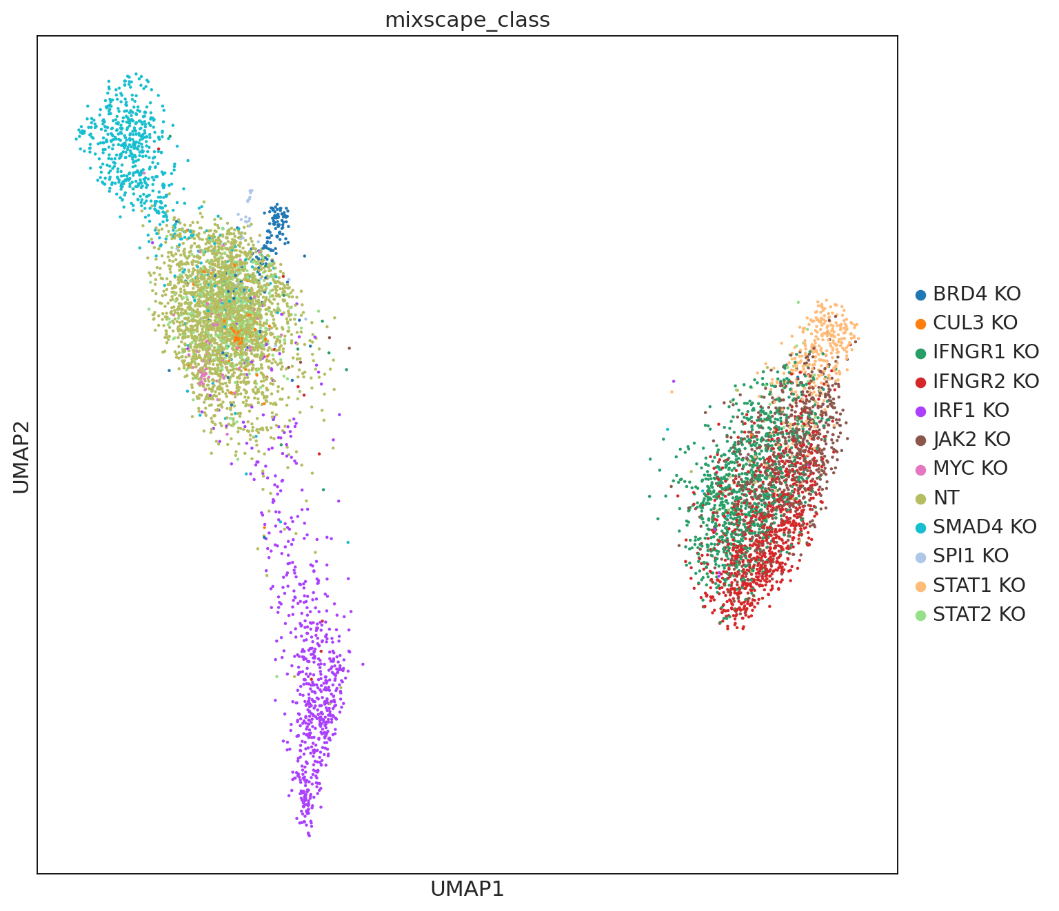
The LDA highlights at least two major types of perturbations as evident by the two islands. However, we want to emphasize that only more stringent analyses, such as pathway analysis followed by biological validation, could determine that several knockouts have similar effects.
Quiz
%run ../src/lib.py

flip_card(
    "q1",
    "Why is it required to have confident cell type labels when applying Augur?",
    "Confident cell type labels are essential when applying Augur because it prioritizes cell types based on their molecular response to perturbations; inaccurate labels can mislead the analysis.",
    back_font_size=15,
)
flip_card(
    "q2",
    "Why should scGen primarily only be applied to highly expressed genes?",
    "scGen should primarily be applied to highly expressed genes, as predicting perturbation responses for lowly expressed genes is challenging due to increased noise and variability.",
    back_font_size=15,
)
flip_card(
    "q3",
    "The mixscape pipeline results in clusters of genetic perturbations. Why must the distances in the UMAPs be interpreted with caution? What does it mean when ome genetic perturbations are close or distant in the UMAP embedding?",
    "In the Mixscape pipeline, distances in UMAP embeddings should be interpreted with caution because they primarily aid visualization; proximity or distance between genetic perturbations in UMAP space doesn't necessarily reflect true biological similarities or differences.",
    front_font_size=15,
    back_font_size=13,
)Contributors
We gratefully acknowledge the contributions of:
Authors
Lukas Heumos
Mohammad Lotfollahi
Reviewers
Yuge Ji
- Srivatsan, S. R., McFaline-Figueroa, J. L., Ramani, V., Saunders, L., Cao, J., Packer, J., Pliner, H. A., Jackson, D. L., Daza, R. M., Christiansen, L., & others. (2020). Massively multiplex chemical transcriptomics at single-cell resolution. Science, 367(6473), 45–51.
- Papalexi, E., Mimitou, E. P., Butler, A. W., Foster, S., Bracken, B., Mauck, W. M., Wessels, H.-H., Hao, Y., Yeung, B. Z., Smibert, P., & Satija, R. (2021). Characterizing the molecular regulation of inhibitory immune checkpoints with multimodal single-cell screens. Nature Genetics, 53(3), 322–331. 10.1038/s41588-021-00778-2
- Frangieh, C. J., Melms, J. C., Thakore, P. I., Geiger-Schuller, K. R., Ho, P., Luoma, A. M., Cleary, B., Jerby-Arnon, L., Malu, S., Cuoco, M. S., & others. (2021). Multimodal pooled Perturb-CITE-seq screens in patient models define mechanisms of cancer immune evasion. Nature Genetics, 53(3), 332–341.
- Replogle, J. M., Saunders, R. A., Pogson, A. N., Hussmann, J. A., Lenail, A., Guna, A., Mascibroda, L., Wagner, E. J., Adelman, K., Bonnar, J. L., & others. (2021). Mapping information-rich genotype-phenotype landscapes with genome-scale Perturb-seq. bioRxiv.
- Wessels, H.-H., Méndez-Mancilla, A., Papalexi, E., Mauck, W. M., Lu, L., Morris, J. A., Mimitou, E., Smibert, P., Sanjana, N. E., & Satija, R. (2022). Efficient combinatorial targeting of term`RNA` transcripts in single cells with Cas13 RNA Perturb-seq. bioRxiv.
- Ji, Y., Lotfollahi, M., Wolf, F. A., & Theis, F. J. (2021). Machine learning for perturbational single-cell omics. Cell Systems, 12(6), 522–537.
- Kang, H. M., Subramaniam, M., Targ, S., Nguyen, M., Maliskova, L., McCarthy, E., Wan, E., Wong, S., Byrnes, L., Lanata, C. M., & others. (2018). Multiplexed droplet single-cell term`RNA`-sequencing using natural genetic variation. Nature Biotechnology, 36(1), 89–94.
- Skinnider, M. A., Squair, J. W., Kathe, C., Anderson, M. A., Gautier, M., Matson, K. J. E., Milano, M., Hutson, T. H., Barraud, Q., Phillips, A. A., Foster, L. J., La Manno, G., Levine, A. J., & Courtine, G. (2021). Cell type prioritization in single-cell data. Nature Biotechnology, 39(1), 30–34. 10.1038/s41587-020-0605-1
- Squair, J. W., Skinnider, M. A., Gautier, M., Foster, L. J., & Courtine, G. (2021). Prioritization of cell types responsive to biological perturbations in single-cell data with Augur. Nature Protocols, 16(8), 3836–3873. 10.1038/s41596-021-00561-x
- Squair, J. W., Gautier, M., Kathe, C., Anderson, M. A., James, N. D., Hutson, T. H., Hudelle, R., Qaiser, T., Matson, K. J. E., Barraud, Q., Levine, A. J., La Manno, G., Skinnider, M. A., & Courtine, G. (2021). Confronting false discoveries in single-cell differential expression. Nature Communications, 12(1), 5692. 10.1038/s41467-021-25960-2
- Bhattacherjee, A., Djekidel, M. N., Chen, R., Chen, W., Tuesta, L. M., & Zhang, Y. (2019). Cell type-specific transcriptional programs in mouse prefrontal cortex during adolescence and addiction. Nature Communications, 10(1), 4169. 10.1038/s41467-019-12054-3
- Lotfollahi, M., Wolf, F. A., & Theis, F. J. (2019). scGen predicts single-cell perturbation responses. Nature Methods, 16(8), 715–721.
- Lotfollahi, M., Naghipourfar, M., Theis, F. J., & Wolf, F. A. (2020). Conditional out-of-distribution generation for unpaired data using transfer VAE. Bioinformatics, 36(Supplement_2), i610–i617.
- Lotfollahi, M., Susmelj, A. K., De Donno, C., Ji, Y., Ibarra, I. L., Wolf, F. A., Yakubova, N., Theis, F. J., & Lopez-Paz, D. (2021). Learning interpretable cellular responses to complex perturbations in high-throughput screens. bioRxiv.
- Russkikh, N., Antonets, D., Shtokalo, D., Makarov, A., Vyatkin, Y., Zakharov, A., & Terentyev, E. (2020). Style transfer with variational autoencoders is a promising approach to term`RNA`-Seq data harmonization and analysis. Bioinformatics, 36(20), 5076–5085.