Gene set enrichment and pathway analysis

Steps

yml

Install conda:
- Before creating the environment, ensure that conda is installed on your system.
Save the yml content:
- Copy the content from the yml tab into a file named environment.yml.
Create the environment:
- Open a terminal or command prompt.
- Run the following command:
```
conda env create -f environment.yml
```
Activate the environment:
- After the environment is created, activate it using:
```
conda activate <environment_name>
```
- Replace <environment_name> with the name specified in the environment.yml file. In the yml file it will look like this:
```
name: <environment_name>
```
Verify the installation:
- Check that the environment was created successfully by running:
```
conda env list
```

gsea_pathway.yml

name: pathway
channels:
  - conda-forge
  - bioconda
dependencies:
  - conda-forge::python=3.12.11
  - conda-forge::r-base=4.4.3
  - conda-forge::pip
  - conda-forge::rpy2=3.6
  - conda-forge::scanpy=1.11.5
  - conda-forge::scikit-misc
  - bioconda::bioconductor-singlecellexperiment=1.28.0
  - bioconda::bioconductor-edger=4.4.0
  - bioconda::bioconductor-limma=3.62.1
  - bioconda::anndata2ri=1.1
  - conda-forge::r-statmod
  - conda-forge::cffi
  - pip:
      - decoupler

Motivation¶

Single-cell RNA-seq provides unprecedented insights into variations in cell types between conditions, tissue types, species and individuals. Differential gene expression analysis of the single-cell data is almost always followed by gene set enrichment analysis, where the aim is to identify gene programs, such as biological processes, gene ontologies or regulatory pathways that are over-represented in an experimental condition compared to control or other conditions, on the basis of differentially expressed (DE) genes.

To determine the pathways enriched in a cell type-specific manner between two conditions, first a relevant collection of gene set signatures is selected, where each gene set defines a biological process (e.g. epithelial to mesenchymal transition, metabolism etc) or pathway (e.g. MAPK signalling). For each gene set in the collection, DE genes present in the gene set are used to obtain a test statistic that is then used to assess the enrichment of the gene set. Depending on the type of the enrichment test chosen, gene expression measurements may or may not be used for the computation of the test statistic.

In this chapter, we first provide an overview of different types of gene set enrichment tests, introduce some commonly used gene signature collections and discuss best practices for pathway enrichment and functional enrichment analysis in general. We conclude the chapter by demonstrating three analytical approaches for gene set enrichment analysis. Note that we use the terms pathway analysis, pathway enrichment analysis, gene set enrichment analysis and functional analysis interchangeably in this chapter.

Pathway and gene set collections¶

Gene sets are a curated list of gene names (or gene ids) that are known to be involved in a biological process through previous studies and/or experiments. The Molecular Signatures Database (MSigDB) Subramanian et al., 2005Liberzon et al., 2011 is the most comprehensive database consisting of 9 collections of gene sets. Some commonly used collections are C5, which is the gene ontology (GO) collection, C2 collection of curated gene signatures from published studies that are typically context (e.g. tissue, condition) specific, but also include KEGG and REACTOME gene signatures. For cancer studies, the Hallmark collection is commonly used, and for immunologic studies the C7 collection is a common choice. Note that these signatures are mainly derived from Bulk-seq measurements and measure continuous phenotypes. Recently and with the wide-spread availability of scRNA-seq datasets, databases have evolved that provide curated marker lists derived from published single cell studies that define cell types in various tissues and species. These include CellMarker Zhang et al., 2019 and PanglaoDB Franzén et al., 2019. Curated marker lists are not limited to those made available in databases, and can be curated by oneself.

Null hypotheses in gene set enrichment analysis¶

Gene set tests can be competitive or self-contained as defined by Goeman and Buhlmann (2007) Goeman & Bühlmann, 2007. Competitive gene set testing tests whether the genes in the set are highly ranked in terms of differential expression relative to the genes not in the set. The sampling unit here is genes, so the test can be done with a single sample (i.e. single-sample GSEA). The test requires genes that are not in the set (i.e background genes). In self-contained gene set testing, the sampling unit is the subject, so multiple samples per group are required, but it is not required to have genes that are not present in the set. A self-contained gene set test tests whether genes in the test set are differentially expressed without regard to any other gene measured in the dataset. These distinctions between the two null hypotheses make differences to the interpretation of gene set enrichment results. Note that in biological data there exist inter-gene correlations, that is the expression of genes in the same pathways are correlated. There are only a few tests that accommodate inter-gene correlations. We will discuss these methods later. Detailed explanations on various gene set tests can be found in limma user manual.

Gene set tests and pathway analysis¶

In scRNA-seq data analysis, gene set enrichment is generally carried out on clusters of cells or cell types, one-at-a-time. Genes differentially expressed in a cluster or cell type are used to identify over-represented gene sets from the selected collection, using simple hypergeometric tests or Fisher’s exact test (as in Enrichr Chen et al., 2013), for example. Such tests do not require the actual gene expression measurements and read counts to compute enrichment statistics, as they rely on testing how significant it is that an $X$ number of genes in a gene set are differentially expressed in the experiment compared to the number of non-DE genes in the set.

fgsea Korotkevich et al., 2021 is a more common tool for gene set enrichment test. fgsea is a computationally faster implementation of the well established Gene Set Enrichment Analysis (GSEA) algorithm Subramanian et al., 2005, which computes enrichment statistics on the basis of some preranked gene-level test statistics. fgsea computes an enrichment score using some signed statistics of the genes in the gene set, such as the t-statistics, log fold-changes (logFC) or p-values from the differential expression test. An empirical (estimated from the data) null distribution is computed for the enrichment score using some random gene sets of the same size, and a p-value is computed to determine the significance of the enrichment score. The p-values are then adjusted for multiple hypothesis testing. GSVA Hänzelmann et al., 2013 is another example of preranked gene set enrichment approaches. We should note that the pre-ranked gene set tests are not specific to single cell datasets and apply to Bulk-seq assays as well.

An alternative approach to test for gene set enrichment in a group of cells, that is clusters or cells of identical types, is to create pseudo-bulk samples from single cells and use gene set enrichment methods developed for Bulk RNA-seq. Several self-contained and competitive gene set enrichment tests, namely fry and camera are implemented in limma Ritchie et al., 2015, which are compatible with the differential gene expression analysis framework through linear models and Empirical Bayes moderation of test statistics Smyth, 2005. Linear models can accommodate complex experimental designs (e.g. subjects, perturbations, batches, nested contrasts, interactions etc) through the design matrix. In addition, the camera and roast gene set tests implemented in limma account for inter-gene correlations. Gene set tests in limma can also be applied to (properly transformed and normalised) single cell measurements without pseudo-bulk generation. However, there are currently no benchmarks that had assessed the accuracy of gene set test results when these methods are applied directly to single cells.

Test	Bulk or SC	Type of Null Hypothesis	Input
Hypergeometric	both	competitive	gene counts
Fisher’s Exact	both	competitive	gene counts
GSEA $^*$	bulk	competitive	gene ranks
GSVA $^*$	bulk	competitive	gene ranks
fgsea	both	competitive	gene ranks
fry $^*$	bulk	self-contained	expression matrix
camera $^*$	bulk	competitive	expression matrix
roast $^*$	bulk	self-contained	expression matrix

Table: Gene set tests, type of the applicable assays and Null Hypothesis they test

$^*$ These tests are practically applicable to single cell datasets, although their application to single cell may not be a common practice.

Gene set test vs. pathway activity inference¶

Gene set tests test whether a pathway is enriched, in other words over-represented, in one condition compared to others, say, in healthy donors compared to severe COVID-19 patients in the monocyte population. An alternative approach is to simply score the activity of a pathway or gene signature, in absolute sense, in individual cells, rather than testing for a differential activity between conditions. Some of the widely used tools for inference of gene set activity in general (including pathway activity) in individual cells include VISION DeTomaso et al., 2019, AUCell Aibar et al., 2017, pathway overdispersion analysis using Pagoda2 Fan et al., 2016Lake et al., 2018 and simple combined z-score Lee et al., 2008.

DoRothEA Garcia-Alonso et al., 2019 and PROGENy Schubert et al., 2018 are among functional analysis tools developed to infer transcription factor (TF) - target activities originally in Bulk RNA data. Holland et al. Holland et al., 2020 found that Bulk RNA-seq methods DoRothEA and PROGENy have optimal performance in simulated scRNA-seq data, and even partially outperform tools specifically designed for scRNA-seq analysis despite the drop-out events and low library sizes in single cell data. Holland et al. also concluded that pathway and TF activity inference is more sensitive to the choice of gene sets rather than the statistical methods. This observation though can be specific to functional enrichment analyses and be explained by the fact that TF-target relations are context-specific; that is TF-target associations in one cell type may actually differ from another cell type or tissue.

In contrast to Holland et al., Zhang et al. Zhang et al., 2020 found that single-cell-based tools, specifically Pagoda2, outperform bulk-based methods from three different aspects of accuracy, stability and scalability. It should be noted that pathway and gene set activity inference tools inherently do not account for batch effects or biological variations other than the biological variation of interest. Therefore, it is up to the data analyst to ensure that the differential gene expression analysis step has worked properly.

Furthermore, while the tools mentioned here score every gene set in individual cells, they are not able to select for the most biologically relevant gene sets among all scored gene sets. scDECAF (https://github.com/DavisLaboratory/scDECAF) is a gene set activity inference tool that allows data-driven selection of the most informative gene sets, thereby aids in dissecting meaningful cellular heterogeneity.

Technical considerations¶

Filtering out the gene sets with low number of genes¶

A common practice is to exclude any gene sets with a few genes overlapping the data or Highly Variable Genes (HVG) in the pre-processing step. Zhang et al. Zhang et al., 2020 found that the performance of both single-cell-based and bulk-based methods drops as gene coverage, that is the number of genes in pathways/gene sets, decreases. Holland et al Holland et al., 2020 also found that gene sets of smaller size adversely impacts the performance of Bulk-seq DoRothEA and PROGENy on single cell data. These report collectively support that filtering gene sets with low gene counts, say less than 10 or 15 genes in the set, is beneficial in pathway analysis. Damian & Gorfine (2004) Damian & Gorfine, 2004 attributed this to the fact gene variances in gene sets with a smaller number of genes are more likely to be large, whereas gene variances in larger gene sets tend to be smaller. This impacts the accuracy of the test statistics computed to test for enrichment. Zhang et al. additionally found that pathway analysis was susceptible to normalization procedures applied to gene expression measurements.

Data normalization¶

Read counts in single cell experiments are typically normalised early on in the pre-processing pipeline to ensure that measurements are comparable across cells of various library sizes. Zhang et al. Zhang et al., 2020 found that normalisation by SCTransform Hafemeister & Satija, 2019 and scran Lun et al., 2016 generally improves the performance of both single-cell- and bulk-based pathway scoring tools. They found that the performance of AUCell (a rank-based method) and z-score (transformation to zero mean, unit standard deviation) is particularly affected by normalization with distinct methods.

Case study: Pathway enrichment analysis and activity level scoring in human PBMC single cells¶

Prepare and explore the data¶

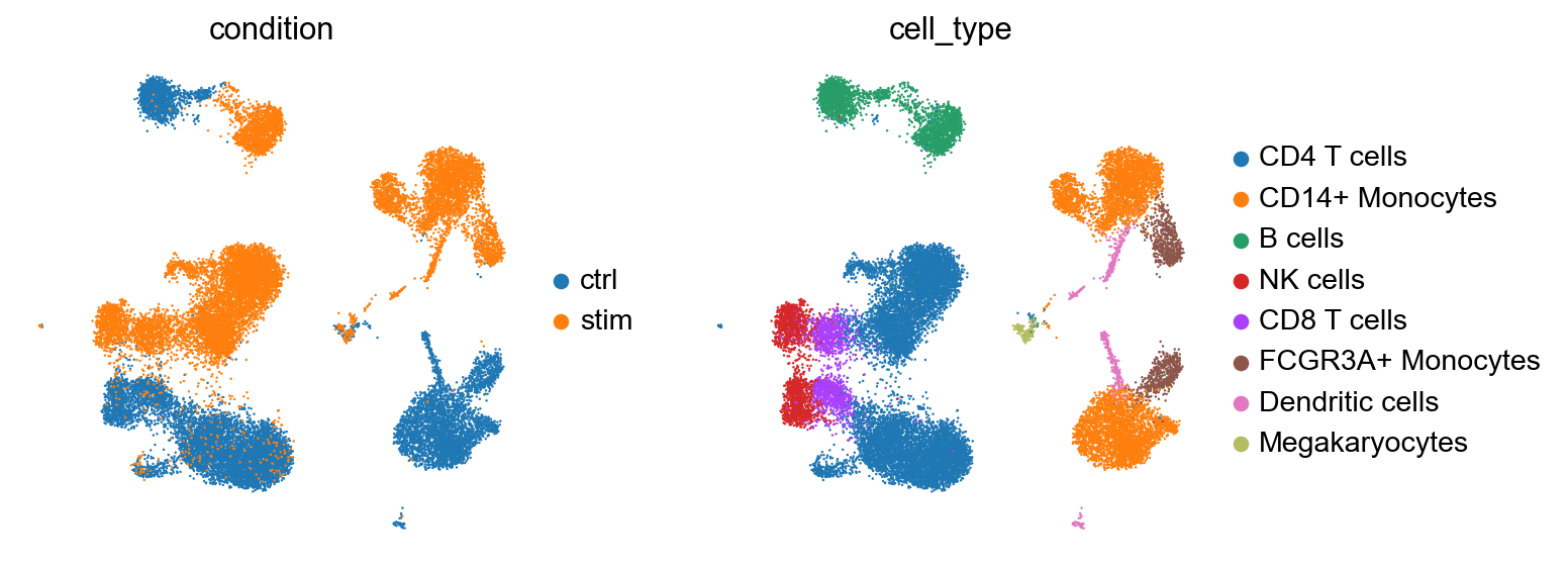
We first download the 25K PBMC data and follow the standard scanpy workflow for normalisation of read counts and subsetting on the highly variable genes. The dataset contains untreated and IFN- $\beta$ stimulated human PBMC cells Kang et al., 2018. We explore patterns of variation in the data with UMAP representation of 4000 highly variable genes.

from __future__ import annotations

import anndata as ad
import decoupler
import numpy as np
import pandas as pd
import scanpy as sc
import seaborn.objects as so
import session_info

sc.settings.set_figure_params(dpi=200, frameon=False)
sc.set_figure_params(dpi=200)
sc.set_figure_params(figsize=(4, 4))

# Filtering warnings from current version of matplotlib
import warnings

warnings.filterwarnings(
    "ignore", message=".*Parameters 'cmap' will be ignored.*", category=UserWarning
)
warnings.filterwarnings(
    "ignore", message="Tight layout not applied.*", category=UserWarning
)

# Setting up R dependencies
import anndata2ri

%load_ext rpy2.ipython

anndata2ri.activate()

%%R
suppressPackageStartupMessages({
    library(SingleCellExperiment)
})

adata = sc.read(
    "kang_counts_25k.h5ad", backup_url="https://figshare.com/ndownloader/files/34464122"
)
adata

AnnData object with n_obs × n_vars = 24673 × 15706
    obs: 'nCount_RNA', 'nFeature_RNA', 'tsne1', 'tsne2', 'label', 'cluster', 'cell_type', 'replicate', 'nCount_SCT', 'nFeature_SCT', 'integrated_snn_res.0.4', 'seurat_clusters'
    var: 'name'
    obsm: 'X_pca', 'X_umap'

# Storing the counts for later use
adata.layers["counts"] = adata.X.copy()
# Renaming label to condition
adata.obs = adata.obs.rename({"label": "condition"}, axis=1)

# Normalizing
sc.pp.normalize_total(adata)
sc.pp.log1p(adata)

# Finding highly variable genes using count data
sc.pp.highly_variable_genes(
    adata, n_top_genes=4000, flavor="seurat_v3", subset=False, layer="counts"
)

adata

AnnData object with n_obs × n_vars = 24673 × 15706
    obs: 'nCount_RNA', 'nFeature_RNA', 'tsne1', 'tsne2', 'condition', 'cluster', 'cell_type', 'replicate', 'nCount_SCT', 'nFeature_SCT', 'integrated_snn_res.0.4', 'seurat_clusters'
    var: 'name', 'highly_variable', 'highly_variable_rank', 'means', 'variances', 'variances_norm'
    uns: 'log1p', 'hvg'
    obsm: 'X_pca', 'X_umap'
    layers: 'counts'

While the current object comes with UMAP and PCA embeddings, these have been corrected for stimulation condition, which we don’t want for this analysis. Instead we will recompute these.

sc.pp.pca(adata)
sc.pp.neighbors(adata)
sc.tl.umap(adata)

/Users/isaac/miniconda3/envs/pathway/lib/python3.9/site-packages/tqdm/auto.py:22: TqdmWarning: IProgress not found. Please update jupyter and ipywidgets. See https://ipywidgets.readthedocs.io/en/stable/user_install.html
  from .autonotebook import tqdm as notebook_tqdm

sc.pl.umap(
    adata,
    color=["condition", "cell_type"],
    frameon=False,
    ncols=2,
)

We generally recommend determining the differentially expressed genes as outlined in the Differential gene expression chapter. For simplicity, here we run a t-test using rank_genes_groups in scanpy to rank genes according to their test statistics for differential expression:

adata.obs["group"] = adata.obs.condition.astype("string") + "_" + adata.obs.cell_type

# find DE genes by t-test
sc.tl.rank_genes_groups(adata, "group", method="t-test", key_added="t-test")

Let’s extract the ranks for genes differentially expressed in response to IFN stimulation in the CD16 Monocyte (FCGR3A+ Monocytes) cluster. We use these ranks and the gene sets from REACTOME to find gene sets enriched in this cell population compared to all other populations using GSEA as implemented in decoupler.

celltype_condition = "stim_FCGR3A+ Monocytes"  # 'stimulated_B',  'stimulated_CD8 T', 'stimulated_CD14 Mono'

# extract scores
t_stats = (
    # Get dataframe of DE results for condition vs. rest
    sc.get.rank_genes_groups_df(adata, celltype_condition, key="t-test")
    # Subset to highly variable genes
    .set_index("names")
    .loc[adata.var["highly_variable"]]
    # Sort by absolute score
    .sort_values("scores", key=np.abs, ascending=False)[
        # Format for decoupler
        ["scores"]
    ]
    .rename_axis(["stim_FCGR3A+ Monocytes"], axis=1)
)
t_stats

Cluster-level gene set enrichment analysis with `decoupler`¶

Now we will use the python package decoupler Mompel et al., 2022 to perform GSEA enrichment tests on our data.

Retrieving gene sets¶

Download and read the gmt file for the REACTOME pathways annotated in the C2 collection of MSigDB.

# Downloading reactome pathways
from pathlib import Path

if not Path("c2.cp.reactome.v7.5.1.symbols.gmt").is_file():
    !wget -O 'c2.cp.reactome.v7.5.1.symbols.gmt' https://figshare.com/ndownloader/files/35233771

def gmt_to_decoupler(pth: Path) -> pd.DataFrame:
    """Parse a gmt file to a decoupler pathway dataframe."""
    from itertools import chain, repeat

    pathways = {}

    with Path(pth).open("r") as f:
        for line in f:
            name, _, *genes = line.strip().split("\t")
            pathways[name] = genes

    return pd.DataFrame.from_records(
        chain.from_iterable(zip(repeat(k), v) for k, v in pathways.items()),
        columns=["geneset", "genesymbol"],
    )

reactome = gmt_to_decoupler("c2.cp.reactome.v7.5.1.symbols.gmt")

Alternatively, we could just query for these resources from omnipath.

However, for stability of this tutorial we are using a fixed version of the gene set collection.

# Retrieving via python
msigdb = decoupler.get_resource("MSigDB")

# Get reactome pathways
reactome = msigdb.query("collection == 'reactome_pathways'")
# Filter duplicates
reactome = reactome[~reactome.duplicated(("geneset", "genesymbol"))]

reactome

Running GSEA¶

First we’ll prepare our gene sets. By default decoupler will not filter gene sets by maximum size, which packages like fgsea do. Instead we will simply manually filter gene sets to have a minimum of 15 genes and a maximum of 500 genes.

# Filtering genesets to match behaviour of fgsea
geneset_size = reactome.groupby("geneset").size()
gsea_genesets = geneset_size.index[(geneset_size > 15) & (geneset_size < 500)]

We’ll use the t-statistics from the t-test to rank the genes for the CD16 Monocyte phenotype upon IFN stimulation and computes p-values for each of the pathways.

scores, norm, pvals = decoupler.run_gsea(
    t_stats.T,
    reactome[reactome["geneset"].isin(gsea_genesets)],
    source="geneset",
    target="genesymbol",
)

gsea_results = (
    pd.concat({"score": scores.T, "norm": norm.T, "pval": pvals.T}, axis=1)
    .droplevel(level=1, axis=1)
    .sort_values("pval")
)

We make a bar plot of top 20 pathways significantly enriched in stimulated CD16 Monocytes compared to all other cell types.

(
    so.Plot(
        data=(
            gsea_results.head(20).assign(
                **{"-log10(pval)": lambda x: -np.log10(x["pval"])}
            )
        ),
        x="-log10(pval)",
        y="source",
    ).add(so.Bar())
)

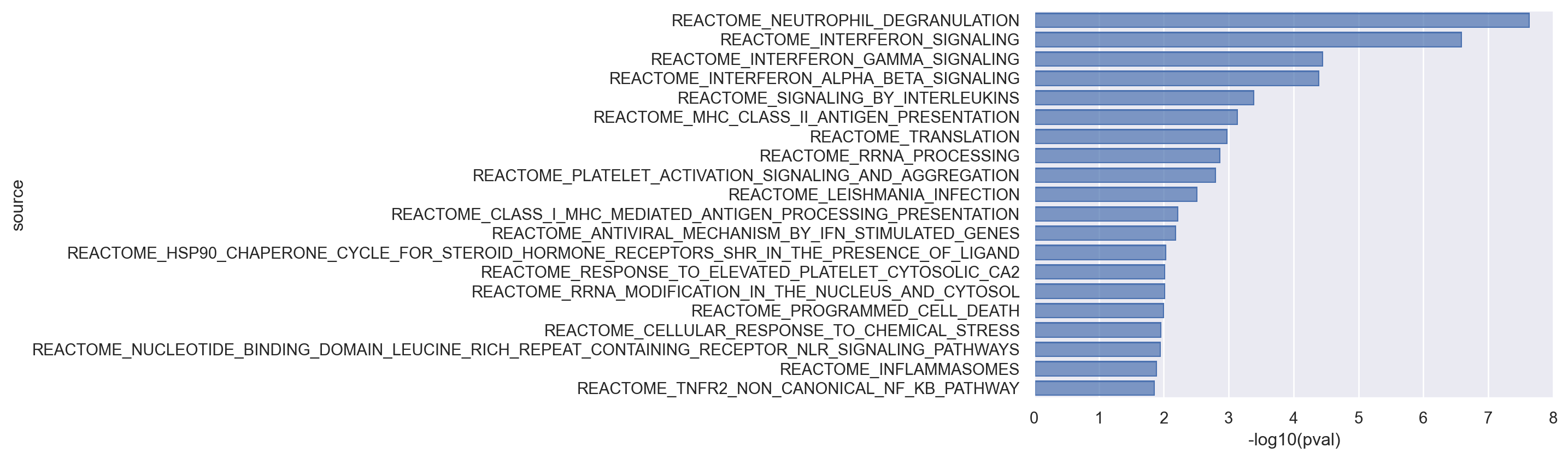
<seaborn._core.plot.Plot at 0x1b5d4e250>

In the plot above, pathway names are given in the y-axis. The x-axis describes the $-\log_{10}$ adjusted p-values. Therefore, the longer the height of the bar, the more significant the pathway is. Pathways are ordered by significance. The majority of interferon-related pathways are indeed ranked among the top 20 most significantly enriched pathways. Some IFN-related pathways include, REACTOME_INTERFERON_SIGNALING (ranked 2nd), REACTOME_INTERFERON_GAMMA_SIGNALING (ranked 3rd), and REACTOME_INTERFERON_ALPHA_BETA_SIGNALING (ranked 4th). Overall, GSEA did a decent job in identifying the pathways known to be associated with interferon signalling, given that we know a priori that IFN-related pathways should be the top-ranked terms.

Let’s look at the raw output of decoupler.mt.gsea:

gsea_results.head(10)

In above, pval is the p-value for the enrichment test, while score and norm are enrichment scores and normalized enrichment scores respectively. Note that enrichment scores are signed. Therefore, a negative score suggests the pathway is down-regulated and a positive score is indicative of up-regulation of genes in the pathway or gene set.

Cell-level pathway activity scoring using AUCell¶

Unlike the previous approach where we assessed gene set enrichment per cluster (or rather cell type), one can score the activity level of pathways and gene sets in each individual cell, that is based on absolute gene expression in the cell, regardless of expression of genes in the other cells. This we can achieve by activity scoring tools such as AUCell.

Similar to GSEA, we will be using the decoupler implementation of AUCell.

%%time
decoupler.run_aucell(
    adata,
    reactome,
    source="geneset",
    target="genesymbol",
    use_raw=False,
)

CPU times: user 16min 42s, sys: 5.09 s, total: 16min 47s
Wall time: 1min 9s

adata

AnnData object with n_obs × n_vars = 24673 × 15706
    obs: 'nCount_RNA', 'nFeature_RNA', 'tsne1', 'tsne2', 'condition', 'cluster', 'cell_type', 'replicate', 'nCount_SCT', 'nFeature_SCT', 'integrated_snn_res.0.4', 'seurat_clusters', 'group'
    var: 'name', 'highly_variable', 'highly_variable_rank', 'means', 'variances', 'variances_norm'
    uns: 'log1p', 'hvg', 'pca', 'neighbors', 'umap', 'condition_colors', 'cell_type_colors', 't-test'
    obsm: 'X_pca', 'X_umap', 'aucell_estimate'
    varm: 'PCs'
    layers: 'counts'
    obsp: 'distances', 'connectivities'

We now add the scores for the interferon-related REACTOME pathways to the obs field of the AnnData object and annotate the activity level of these pathways in each of the cells on the UMAP:

ifn_pathways = [
    "REACTOME_INTERFERON_SIGNALING",
    "REACTOME_INTERFERON_ALPHA_BETA_SIGNALING",
    "REACTOME_INTERFERON_GAMMA_SIGNALING",
]

adata.obs[ifn_pathways] = adata.obsm["aucell_estimate"][ifn_pathways]

Plot the scores on the umap

sc.pl.umap(
    adata,
    color=["condition", "cell_type"] + ifn_pathways,
    frameon=False,
    ncols=2,
    wspace=0.3,
)

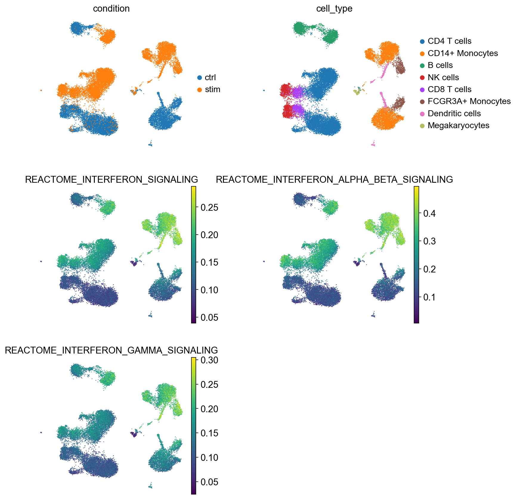
AUCell scores the pathways well-known to be implicated in interferon signalling high in IFN-stimulated cells, while cells in the control condition generally have low scores for these pathways, demonstrating that gene set scoring with AUCell has been successful. Also note that the scores are generally larger for terms that are ranked higher in the gene set enrichment test results by GSEA. The concordance between pathway activity scores by AUCell and gene set enrichment test by GSEA is promising, given that we know a priori that IFN-related pathways should be the top-ranked terms. In addition, the effect of IFN stimulation is very large in this dataset and this contributes to the performance of the methods here.

Gene set enrichment for complex experimental designs using limma-fry and pseudo-bulks¶

In cluster-level t-test approach, differentially expressed genes are found by comparing a cluster to all other clusters, which in this case includes both control and stimulated cells. Linear models allow us to compare cells in the stimulated condition only to those in the control group, resulting in more accurate identification of genes responding to the stimulus. Indeed, linear models can accommodate for complex experimental designs, for example, identification of gene sets enriched in Cell type A in treatment 1 compared to Cell type A in treatment 2; that is, across perturbation and across cell types effects, while adjusting for batch effects, between-individual variations, gender and strain differences in mouse models etc.

In the next section, we demonstrate a limma-fry workflow that generalize to realistic data analysis routines, say, for single-cell case control studies. We first create pseudo-bulk replicates per cell type and condition (3 replicates per condition - cell type combination). We then find gene sets enriched in stimulated compared to control cells in a cell type. We also assess gene set enrichment between two stimulated cell type populations to find differences in signalling pathways.

Create pseudo-bulk samples and explore the data¶

def subsampled_summation(
    adata: ad.AnnData,
    groupby: str | list[str],
    *,
    n_samples_per_group: int,
    n_cells: int,
    random_state: None | int | np.random.RandomState = None,
    layer: str = None,
) -> ad.AnnData:
    """Sum sample of X per condition.

    Drops conditions which don't have enough samples.

    Parameters
    ----------
    adata
        AnnData to sum expression of
    groupby
        Keys in obs to groupby
    n_samples_per_group
        Number of samples to take per group
    n_cells
        Number of cells to take per sample
    random_state
        Random state to use when sampling cells
    layer
        Which layer of adata to use

    Returns:
    -------
    AnnData with same var as original, obs with columns from groupby, and X.
    """
    from scipy import sparse
    from sklearn.utils import check_random_state

    # Checks
    if isinstance(groupby, str):
        groupby = [groupby]
    random_state = check_random_state(random_state)

    indices = []
    labels = []

    grouped = adata.obs.groupby(groupby)
    for k, inds in grouped.indices.items():
        # Check size of group
        if len(inds) < (n_cells * n_samples_per_group):
            continue

        # Sample from group
        condition_inds = random_state.choice(
            inds, n_cells * n_samples_per_group, replace=False
        )
        for i, sample_condition_inds in enumerate(np.split(condition_inds, 3)):
            if isinstance(k, tuple):
                labels.append((*k, i))
            else:  # only grouping by one variable
                labels.append((k, i))
            indices.append(sample_condition_inds)

    # obs of output AnnData
    new_obs = pd.DataFrame.from_records(
        labels,
        columns=[*groupby, "sample"],
        index=["-".join(map(str, l)) for l in labels],
    )
    n_out = len(labels)

    # Make indicator matrix
    indptr = np.arange(0, (n_out + 1) * n_cells, n_cells)
    indicator = sparse.csr_matrix(
        (
            np.ones(n_out * n_cells, dtype=bool),
            np.concatenate(indices),
            indptr,
        ),
        shape=(len(labels), adata.n_obs),
    )

    return ad.AnnData(
        X=indicator @ sc.get._get_obs_rep(adata, layer=layer),
        obs=new_obs,
        var=adata.var.copy(),
    )

pb_data = subsampled_summation(
    adata, ["cell_type", "condition"], n_cells=75, n_samples_per_group=3, layer="counts"
)
pb_data

AnnData object with n_obs × n_vars = 42 × 15706
    obs: 'cell_type', 'condition', 'sample'
    var: 'name', 'highly_variable', 'highly_variable_rank', 'means', 'variances', 'variances_norm'

# Does PC1 captures a meaningful biological or technical fact?
pb_data.obs["lib_size"] = pb_data.X.sum(1)

Let’s normalize this data and take a quick look at it. We won’t use a neighbor embedding here since the sample size is significantly reduced.

pb_data.layers["counts"] = pb_data.X.copy()

sc.pp.normalize_total(pb_data)
sc.pp.log1p(pb_data)
sc.pp.pca(pb_data)

sc.pl.pca(pb_data, color=["cell_type", "condition", "lib_size"], ncols=1, size=250)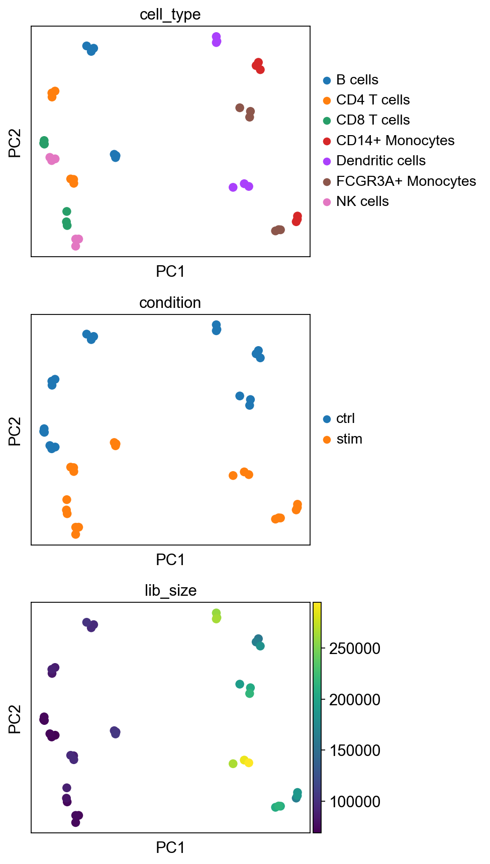

PC1 now captures difference between lymphoid (T, NK, B) and myeloid (Mono, DC) populations, while the second PC captures variation due to administration of stimulus (i.e. difference between control and stimulated pseudo-replicates). Ideally, the variation of interest has to be detectable in top few PCs of the pseudo-bulk data.

In this case, since we are indeed interested in stimulation effect per cell type, we proceed to gene set testing. We re-iterate that the purpose of plotting PCs is to explore various axes of variability in the data and to spot unwanted variabilities that can substantially influence the test results. Users may proceed with the rest of the analyses should they be satisfied with the variations in their data.

Setup for `limma` and `fry`¶

For this next part of the analysis we will be using Bioconductor packages limma and it’s method fry.

We first set up the design and contrast matrices. Let’s remind ourselves that a design matrix is a mathematical representation of group membership (i.e. the group or condition to which a sample belongs), and contrast matrices are mathematical representations of comparisons of interest for the differential test.

groups = pb_data.obs.condition.astype("string") + "_" + pb_data.obs.cell_type

%%R -i groups
group <-  as.factor(gsub(" |\\+","_", groups))
design <- model.matrix(~ 0 + group)
head(design)

     [,1] [,2] [,3] [,4] [,5] [,6] [,7] [,8] [,9] [,10] [,11] [,12] [,13] [,14]
[1,]    0    0    1    0    0    0    0    0    0     0     0     0     0     0
[2,]    0    0    1    0    0    0    0    0    0     0     0     0     0     0
[3,]    0    0    1    0    0    0    0    0    0     0     0     0     0     0
[4,]    0    0    0    0    0    0    0    0    0     1     0     0     0     0
[5,]    0    0    0    0    0    0    0    0    0     1     0     0     0     0
[6,]    0    0    0    0    0    0    0    0    0     1     0     0     0     0

%%R
colnames(design)

 [1] "groupctrl_B_cells"           "groupctrl_CD14__Monocytes"  
 [3] "groupctrl_CD4_T_cells"       "groupctrl_CD8_T_cells"      
 [5] "groupctrl_Dendritic_cells"   "groupctrl_FCGR3A__Monocytes"
 [7] "groupctrl_NK_cells"          "groupstim_B_cells"          
 [9] "groupstim_CD14__Monocytes"   "groupstim_CD4_T_cells"      
[11] "groupstim_CD8_T_cells"       "groupstim_Dendritic_cells"  
[13] "groupstim_FCGR3A__Monocytes" "groupstim_NK_cells"

%%R 
kang_pbmc_con <- limma::makeContrasts(
    
    # the effect if stimulus in CD16 Monocyte cells
    groupstim_FCGR3A__Monocytes - groupctrl_FCGR3A__Monocytes,
    
    # the effect of stimulus in CD16 Monocytes compared to CD8 T Cells
    (groupstim_FCGR3A__Monocytes - groupctrl_FCGR3A__Monocytes) - (groupstim_CD8_T_cells - groupctrl_CD8_T_cells), 
    levels = design
)

Index the genes annotated in each pathway in our data as follows:

log_norm_X = pb_data.to_df().T

%%R -i log_norm_X -i reactome
# Move pathway info from python to R
pathways = split(reactome$genesymbol, reactome$geneset)
# Map gene names to indices
idx = limma::ids2indices(pathways, rownames(log_norm_X))

/Users/isaac/miniconda3/envs/pathway/lib/python3.9/site-packages/rpy2/robjects/pandas2ri.py:54: FutureWarning: iteritems is deprecated and will be removed in a future version. Use .items instead.
  for name, values in obj.iteritems():
/Users/isaac/miniconda3/envs/pathway/lib/python3.9/site-packages/rpy2/robjects/pandas2ri.py:54: FutureWarning: iteritems is deprecated and will be removed in a future version. Use .items instead.
  for name, values in obj.iteritems():

As done in the gsea method, let’s remove gene sets with less than 15 genes

%%R
keep_gs <- lapply(idx, FUN=function(x) length(x) >= 15)
idx <- idx[unlist(keep_gs)]

Now that we have set up the design and contrast matrices, and have indexed the genes in each pathway in our data, we can call fry() to test for enriched pathways in each of the contrasts we set above:

fry test for Stimulated vs Control¶

%%R -o fry_results
fry_results <- limma::fry(log_norm_X, index = idx, design = design, contrast = kang_pbmc_con[,1])

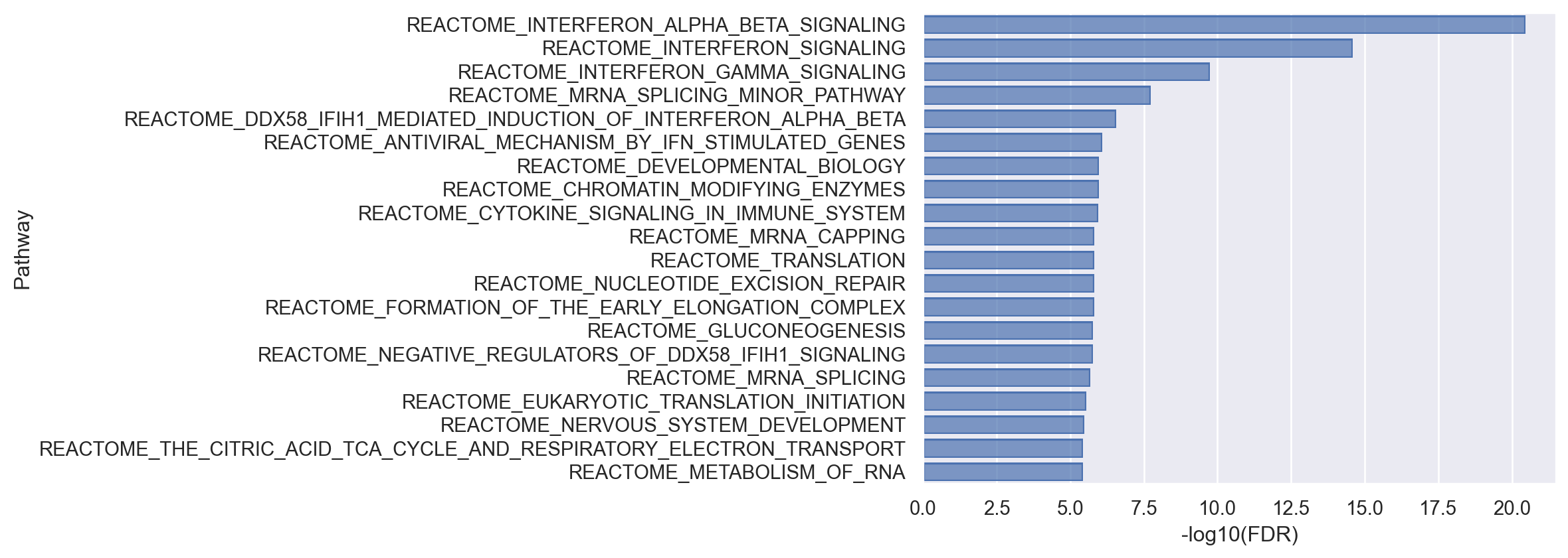
Taking a look at the top ranked pathways we’ll see some familiar names:

fry_results.head()

(
    so.Plot(
        data=(
            fry_results.head(20)
            .assign(**{"-log10(FDR)": lambda x: -np.log10(x["FDR"])})
            .rename_axis(index="Pathway")
        ),
        x="-log10(FDR)",
        y="Pathway",
    ).add(so.Bar())
)

<seaborn._core.plot.Plot at 0x1b7940970>

fry test for the comparison between two stimulated cell types¶

%%R -o fry_results_negative_ctrl
fry_results_negative_ctrl <- limma::fry(log_norm_X, index = idx, design = design, contrast = kang_pbmc_con[,2])

(
    so.Plot(
        data=(
            fry_results_negative_ctrl.head(20)
            .assign(**{"-log10(FDR)": lambda x: -np.log10(x["FDR"])})
            .rename_axis(index="Pathway")
        ),
        x="-log10(FDR)",
        y="Pathway",
    ).add(so.Bar())
)

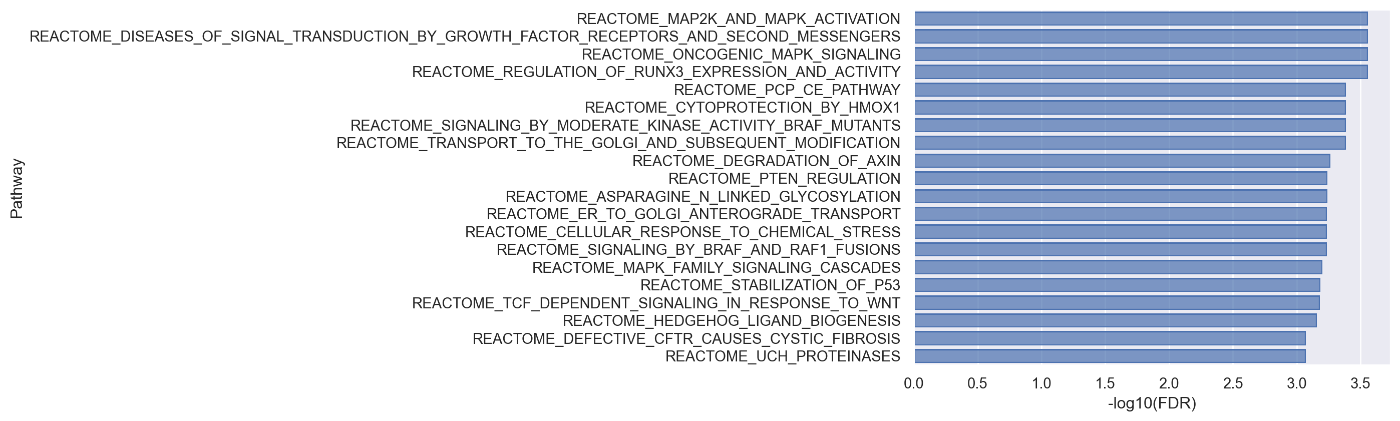
<seaborn._core.plot.Plot at 0x1b81a2be0>

As demonstrated above, limma-fry can accommodate gene set enrichment tests for datasets and research problems with complex experimental designs. Both gsea and fry provide insights into the direction of enrichment (positive or negative score in gsea and Direction field in fry). They both can be applied to clusters of cells or pseudo-bulk samples. However, Unlike gsea, more flexible tests can be carried out with fry. In addition, fry can reveal if genes in a pathway are changing between the experimental conditions but in consistent or inconsistent directions. Pathways in which the genes change in consistent direction are identified with FDR < 0.05. Pathways in which the genes are DE between the conditions but they change in different, inconsistent directions can be identified where FDR > 0.05, but FDR.Mixed < 0.05 (assuming 0.05 is the desired significance level). fry is bidirectional, applicable to arbitrary designs and works well with small number of samples (although this may not be an issue in single cell). Therefore, the results by fry might be of more interest biologically.

On the effect of filtering low-expression genes¶

As mentioned before, Ideally, the variation of interest has to be detectable in top few PCs of the pseudo-bulk data. Let’s remove genes with low expression in the data, apply $\log_2$ CPM transformation and repeat the PCA plots:

counts_df = pb_data.to_df(layer="counts").T

%%R -i counts_df
keep <- edgeR::filterByExpr(counts_df) # in real analysis, supply the desig matrix to the function to retain as more genes as possible
counts_df <- counts_df[keep,]
logCPM <- edgeR::cpm(counts_df, log=TRUE, prior.count = 2)

/Users/isaac/miniconda3/envs/pathway/lib/python3.9/site-packages/rpy2/robjects/pandas2ri.py:54: FutureWarning: iteritems is deprecated and will be removed in a future version. Use .items instead.
  for name, values in obj.iteritems():
R[write to console]: No group or design set. Assuming all samples belong to one group.

%%R -o logCPM
logCPM = data.frame(logCPM)

pb_data.uns["logCPM_FLE"] = logCPM.T  # FLE for filter low exprs

pb_data.obsm["logCPM_FLE_pca"] = sc.pp.pca(logCPM.T.to_numpy(), return_info=False)

sc.pl.embedding(pb_data, "logCPM_FLE_pca", color=pb_data.obs, ncols=1, size=250)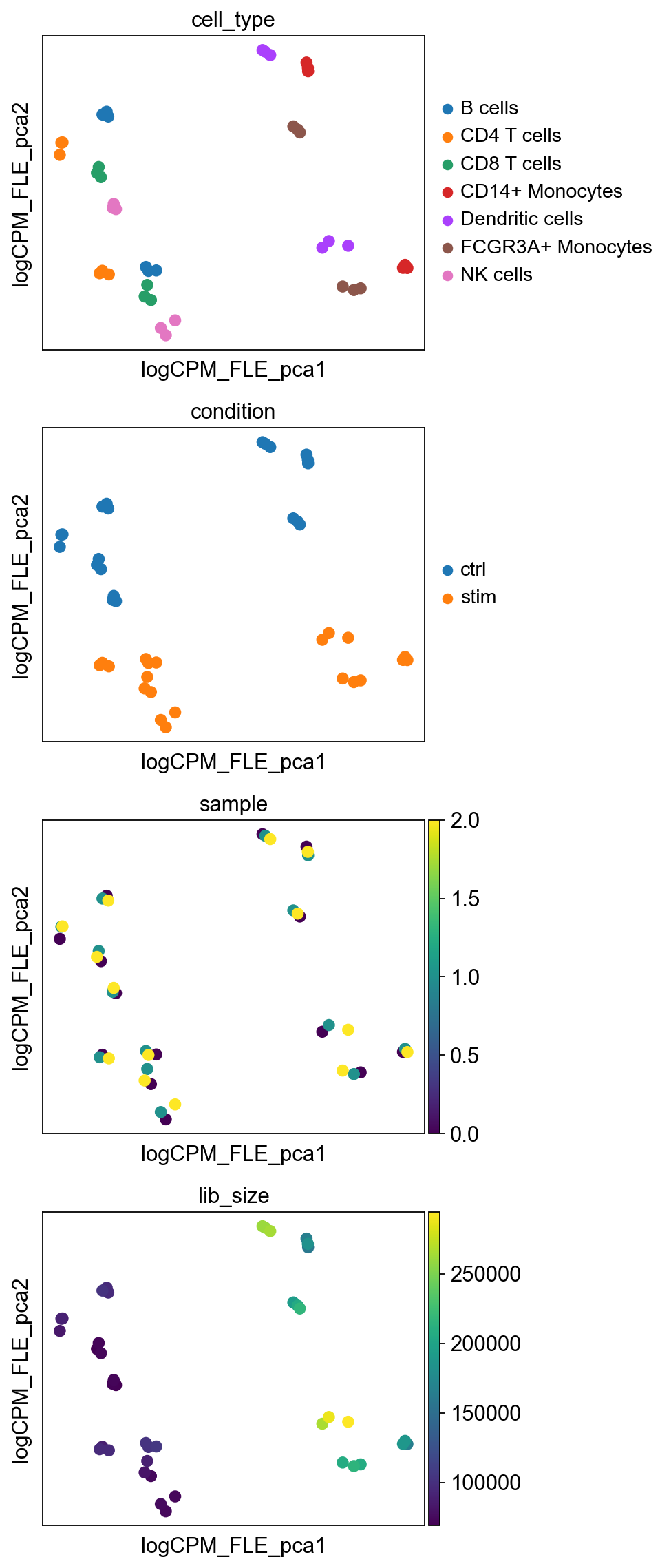

Here, “logCPM_FLE” denotes filtering for low expressed genes followed by $\log_2$ CPM transformation. We can now clearly observe that PC1 captures cell type effect and PC2 captures the treatment effect, when low-expressed genes are removed and differences between library sizes are adjusted by $\log_2$ CPM transformation.

Since in this case study we are indeed interested in stimulation effect per cell type, and this variation is better preserved before gene filtering, we presented the enrichment test results on unfiltered data. In practice, filtering low abundance genes and computation of normalisation factors by edgeR::calcNormFactors are standard part of bulk RNA-seq analysis workflow. Should we have been interested in global effects of IFN stimulation, we should have used the filtered data. Additionally, one can note that design <- model.matrix(~ 0 + lineage + group) would take into account differences (that is baseline expression differences) between myeloid and lymphoid lineages, improving the separation of pseudo-bulk samples by IFN stimulation, possibly along PC1. In this case study, we were interested in cell type-specific effects, hence we stayed with a model of data whereby the variability along PC1 is by cell type. The choice of design matrix has to be carefully considered to align with the biological question of interest.

A note on the redundancy between gene sets and the performance of preranked and fry gene set tests¶

Generally, there can be a large overlap between closely related gene sets. This overlap impacts the rank of the gene sets in the enrichment results and can compromise the final interpretation. For example, the cells in Kang et al. are treated with IFN- $\beta$ . Therefore, one would expect to see the term REACTOME_INTERFERON_ALPHA_BETA_SIGNALING as the top ranked term. While this term is indeed the top rank term in the output of fry, in the output of GSEA REACTOME_INTERFERON_SIGNALING is the top rank term. This term has a larger number of genes (52) compared to REACTOME_INTERFERON_ALPHA_BETA_SIGNALING (24 genes), and most of those genes are shared between the two terms. This illustrates another difference between preranked gene set tests such as GSEA and fry, in preventing the larger gene sets from dominating the enrichment results. The better performance of fry is due to more accurate estimation of gene expression variances, hence more sensitive DE gene results.

Quiz¶

%run ../src/lib.py

flip_card(
    "q1",
    "What is the difference between gene set enrichment tests and activity scoring?",
    "Gene set enrichment tests focus on identifying gene sets that are overrepresented among differentially expressed genes. Activity scoring assesses the activity level of a pathway within individual samples by summarizing the expression of genes in a set, providing a continuous score that reflects pathway activity.",
    back_font_size=12,
)
flip_card(
    "q2",
    "Describe examples of settings where gene set tests should be used. Can you outline examples of settings where pathway activity scoring methods are applicable?",
    "Gene Set Tests are aplicable when comparing groups of samples to identify pathways differentially expressed between conditions, such as treated versus untreated groups. Pathway Activity Scoring Methods are useful for single-sample analyses to determine pathway activity levels within individual samples, aiding in personalized medicine or when sample sizes are limited.",
    back_font_size=10,
)
flip_card(
    "q3",
    "What are the two types of Null Hypothesis in gene set enrichment tests? Explain the difference between the two types.",
    "Competitive Null Hypothesis: Posits that genes within the set are not more associated with the phenotype than those outside the set. The test compares the association of genes inside the set to those outside. Self-contained Null Hypothesis: Asserts that no genes in the set are associated with the phenotype. The test evaluates the gene set independently, without considering genes outside the set.",
    back_font_size=10,
)
flip_card(
    "q4",
    "What is the most important preprocessing step in pathway analysis? What are the consequences if it is not conducted properly?",
    "Proper normalization of gene expression data is crucial. Inadequate normalization can lead to misleading results, as technical variations may be mistaken for biological differences, affecting the accuracy of pathway analysis.",
    back_font_size=12,
)
flip_card(
    "q5",
    "Name one gene set testing and one gene set activity scoring algorithm and explain it briefly.",
    "Gene Set Enrichment Analysis (GSEA) evaluates whether predefined gene sets show statistically significant, concordant differences between two biological states. Single-sample GSEA (ssGSEA) computes separate enrichment scores for each pairing of a sample and gene set, transforming gene expression data into pathway activity profiles for individual samples.",
    back_font_size=12,
)

Session info¶

%%R
sessionInfo()

R version 4.1.2 (2021-11-01)
Platform: x86_64-apple-darwin13.4.0 (64-bit)
Running under: macOS Big Sur 11.6.8

Matrix products: default
LAPACK: /Users/isaac/miniconda3/envs/pathway/lib/libopenblasp-r0.3.21.dylib

locale:
[1] C/UTF-8/C/C/C/C

attached base packages:
[1] stats4    tools     stats     graphics  grDevices utils     datasets 
[8] methods   base     

other attached packages:
 [1] SingleCellExperiment_1.16.0 SummarizedExperiment_1.24.0
 [3] Biobase_2.54.0              GenomicRanges_1.46.1       
 [5] GenomeInfoDb_1.30.1         IRanges_2.28.0             
 [7] S4Vectors_0.32.4            BiocGenerics_0.40.0        
 [9] MatrixGenerics_1.6.0        matrixStats_0.63.0         

loaded via a namespace (and not attached):
 [1] Rcpp_1.0.9             locfit_1.5-9.6         edgeR_3.36.0          
 [4] lattice_0.20-45        bitops_1.0-7           grid_4.1.2            
 [7] zlibbioc_1.40.0        XVector_0.34.0         limma_3.50.1          
[10] Matrix_1.5-3           statmod_1.4.37         RCurl_1.98-1.9        
[13] DelayedArray_0.20.0    compiler_4.1.2         GenomeInfoDbData_1.2.7

session_info.show()

Contributors¶

We gratefully acknowledge the contributions of:

Authors¶

Lukas Heumos
Anastasia Litinetskaya
Soroor Hediyeh-Zadeh

Reviewers¶

References¶

Subramanian, A., Tamayo, P., Mootha, V. K., Mukherjee, S., Ebert, B. L., Gillette, M. A., Paulovich, A., Pomeroy, S. L., Golub, T. R., Lander, E. S., & others. (2005). Gene set enrichment analysis: a knowledge-based approach for interpreting genome-wide expression profiles. Proceedings of the National Academy of Sciences, 102(43), 15545–15550.
Liberzon, A., Subramanian, A., Pinchback, R., Thorvaldsdóttir, H., Tamayo, P., & Mesirov, J. P. (2011). Molecular signatures database (MSigDB) 3.0. Bioinformatics, 27(12), 1739–1740.
Zhang, X., Lan, Y., Xu, J., Quan, F., Zhao, E., Deng, C., Luo, T., Xu, L., Liao, G., Yan, M., & others. (2019). CellMarker: a manually curated resource of cell markers in human and mouse. Nucleic Acids Research, 47(D1), D721–D728.
Franzén, O., Gan, L.-M., & Björkegren, J. L. (2019). PanglaoDB: a web server for exploration of mouse and human single-cell RNA sequencing data. Database, 2019.
Goeman, J. J., & Bühlmann, P. (2007). Analyzing gene expression data in terms of gene sets: methodological issues. Bioinformatics, 23(8), 980–987.
Chen, E. Y., Tan, C. M., Kou, Y., Duan, Q., Wang, Z., Meirelles, G. V., Clark, N. R., & Ma’ayan, A. (2013). Enrichr: interactive and collaborative HTML5 gene list enrichment analysis tool. BMC Bioinformatics, 14(1), 1–14.
Korotkevich, G., Sukhov, V., Budin, N., Shpak, B., Artyomov, M. N., & Sergushichev, A. (2021). Fast gene set enrichment analysis. BioRxiv, 060012.
Hänzelmann, S., Castelo, R., & Guinney, J. (2013). GSVA: gene set variation analysis for microarray and RNA-seq data. BMC Bioinformatics, 14(1), 1–15.
Ritchie, M. E., Phipson, B., Wu, D., Hu, Y., Law, C. W., Shi, W., & Smyth, G. K. (2015). limma powers differential expression analyses for RNA-sequencing and microarray studies. Nucleic Acids Research, 43(7), e47–e47.
Smyth, G. K. (2005). Limma: linear models for microarray data. In Bioinformatics and computational biology solutions using R and Bioconductor (pp. 397–420). Springer.
DeTomaso, D., Jones, M. G., Subramaniam, M., Ashuach, T., Ye, C. J., & Yosef, N. (2019). Functional interpretation of single cell similarity maps. Nature Communications, 10(1), 1–11.
Aibar, S., González-Blas, C. B., Moerman, T., Huynh-Thu, V. A., Imrichova, H., Hulselmans, G., Rambow, F., Marine, J.-C., Geurts, P., Aerts, J., & others. (2017). SCENIC: single-cell regulatory network inference and clustering. Nature Methods, 14(11), 1083–1086.
Fan, J., Salathia, N., Liu, R., Kaeser, G. E., Yung, Y. C., Herman, J. L., Kaper, F., Fan, J.-B., Zhang, K., Chun, J., & others. (2016). Characterizing transcriptional heterogeneity through pathway and gene set overdispersion analysis. Nature Methods, 13(3), 241–244.
Lake, B. B., Chen, S., Sos, B. C., Fan, J., Kaeser, G. E., Yung, Y. C., Duong, T. E., Gao, D., Chun, J., Kharchenko, P. V., & others. (2018). Integrative single-cell analysis of transcriptional and epigenetic states in the human adult brain. Nature Biotechnology, 36(1), 70–80.
Lee, E., Chuang, H.-Y., Kim, J.-W., Ideker, T., & Lee, D. (2008). Inferring pathway activity toward precise disease classification. PLoS Computational Biology, 4(11), e1000217.