RNA velocity - Single-cell best practices

Steps

yml

Install conda:
- Before creating the environment, ensure that conda is installed on your system.
Save the yml content:
- Copy the content from the yml tab into a file named environment.yml.
Create the environment:
- Open a terminal or command prompt.
- Run the following command:
```
conda env create -f environment.yml
```
Activate the environment:
- After the environment is created, activate it using:
```
conda activate <environment_name>
```
- Replace <environment_name> with the name specified in the environment.yml file. In the yml file it will look like this:
```
name: <environment_name>
```
Verify the installation:
- Check that the environment was created successfully by running:
```
conda env list
```

rna_velocity.yml

name: rna_velocity
channels:
  - defaults
  - conda-forge
dependencies:
  - conda-forge::python=3.13
  - conda-forge::ipykernel=7.2.0
  - conda-forge::scvelo=0.3.3
  - pip
  - pip:
      - lamindb

This book uses lamindb to store, share, and load datasets and notebooks using the theislab/sc-best-practices instance. We acknowledge free hosting from Lamin Labs.

Install lamindb
- Install the lamindb Python package:
```
pip install lamindb
```
Optionally create a lamin account
- Sign up and log in following the instructions
Verify your setup
- Run the lamin connect command:
```
import lamindb as ln

ln.Artifact.connect("theislab/sc-best-practices").df()
```
You should now see up to 100 of the stored datasets.
Accessing datasets (Artifacts)
- Search for the datasets on the Artifacts page
- Load an Artifact and the corresponding object:
```
import lamindb as ln
af = ln.Artifact.connect("theislab/sc-best-practices").get(key="key_of_dataset", is_latest=True)
obj = af.load()
```
The object is now accessible in memory and is ready for analysis. Adapt the lamindb.Artifact.connect("theislab/sc-best-practices").get("SOMEIDXXXX") suffix to get respective versions.
Accessing notebooks (Transforms)
- Search for the notebook on the Transforms page
- Load the notebook:
```
lamin load <notebook url>
```
which will download the notebook to the current working directory. Analogously to Artifacts, you can adapt the suffix ID to get older versions.

Motivation¶

Single-cell datasets enable the study of biological processes, such as early development, at high resolution. While single cells are analysed instead of a tissue as a whole, for example, changes in cells’ phenotypic traits cannot be tracked over time. This fact stems from the destructive nature of single-cell sequencing protocols. Upon sequencing a cell, it is destroyed, and its defining characteristics can therefore not be measured again at a later time point. Notably, experimental techniques not only fail to measure the general cellular profile at different times but also how quickly these changes take place. Recovering the position in time along the developmental landscape can be achieved with tools from the field of trajectory inference (TI). However, classical TI methods do not offer any directed, dynamic information. Additionally, these algorithms typically do not account for information beyond transcriptomic reads and similarity.

Modeling RNA velocity¶

The change in the transcriptomic profile of a cell is triggered by a cascade of events: Broadly speaking, DNA is transcribed to produce so-called unspliced precursor messenger RNA (pre-mRNA). Unspliced pre-mRNA contains regions relevant for translation (exons) as well as non-coding regions (introns). These non-coding regions are spliced out, i.e., removed, to form spliced, mature mRNA. While single-cell RNA sequencing (scRNA-seq) protocols fail to capture the transcriptome at multiple timepoints, they do include the necessary information to disassociate unspliced and spliced mRNA reads Manno et al., 2018Srivastava et al., 2019He et al., 2022Melsted et al., 2021.

Identifying unspliced and spliced reads allows formulating a dynamical model describing splicing kinetics Zeisel et al., 2011 and inferring the corresponding model weights based on single cell data. The change in spliced RNA described by the model is called RNA velocity Manno et al., 2018. Current models of RNA velocity assume the gene-specific model

\begin{aligned} \frac{du_g}{dt} &= \alpha_g - \beta_g u_g\\ \frac{ds_g}{dt} &= \beta_g u_g - \gamma_g s_g, \end{aligned}

(1)

with transcription rate $\alpha_g$ , splicing rate $\beta_g$ , and degradation rate $\gamma_g$ of spliced RNA. While the kinetics of each gene are modelled independently of each other, we will drop the index $g$ for notational simplicity. Even though the field of parameter estimation in dynamical systems is well studied, inference algorithms require the time per observation to be known. Consequently, these traditional methods cannot be applied to infer RNA velocity and its model parameters from scRNA-seq data.

Parameter inference¶

Single-cell measurements are snapshot data and cannot, therefore, be plotted against time. Instead, classical RNA velocity methods rely on studying the cell-specific tuples $(u, s)$ of unspliced and spliced RNA for each gene. The collection of these tuples forms the so-called phase portrait. Assuming constant rates of transcription, splicing, and degradation, the phase portraits exhibit an almond shape. The upper arc corresponds to the induction, the lower arc to the repression phase. However, as real-world data is noisy, plotting the unspliced against spliced counts does not recover the expected almond shape. Instead, the data needs to be smoothed first. Classically, this preprocessing step consists of averaging the gene expression of each cell over its neighbors in a cell-cell similarity graph.

The steady-state model¶

The first attempt at estimating RNA velocity assumed gene independence and the underlying kinetics to be governed by the above model. Additionally, it is assumed that (1) kinetics have reached their equilibrium, (2) rates are constant, and (3) there is a single, common splicing rate across all genes. In the following, we will refer to this model as the steady-state model due to the first assumption. The steady-states themselves are found in the upper right corner of the phase portrait (induction phase) and their origin (repression phase). Based on these extreme quantiles, the steady-state model estimates the steady-state ratio with a linear regression fit. RNA velocity is then defined as the residual to this fit.

Even though the steady-state model can successfully recover the developmental direction in some systems, it is inherently limited by its model assumptions. The two assumptions that are readily violated are the common splicing rate across genes and the assumption that the equilibria are observed during the experiment. Consequently, inference in these cases will yield incorrect results. Additionally, the steady-state model only considers a subset of the data, and only the steady-state ratio but not each model parameter is inferred.

The EM model¶

To overcome the limitations of the steady-state model, several extensions have been proposed. The so-far most popular one is the EM model implemented in scVelo Bergen et al., 2020. The EM model no longer assumes that steady-states have been reached or that genes share a common splicing rate. Additionally, all datapoints are used to infer the full set of parameters as well as a gene and cell-specific latent time of the splicing model. The algorithm uses an expectation-maximization (EM) framework to estimate parameters. The unobserved variables in the E-step are each cell’s time and state (induction, repression, or steady-state). All other model parameters are inferred during the M-step.

While the EM model no longer relies on key assumptions of the steady-state model and, thus, is more broadly applicable, the inferred RNA velocity may still violate prior biological knowledge Bergen et al., 2021, Barile et al., 2021. The reason for such failure cases are mainly two-fold: On the one hand, the EM model continues to assume constant rates. Consequently, whenever these assumptions do not hold, for example, in erythroid maturation Barile et al., 2021, the inference is incorrect. On the other hand, the proposed model relies on phase portraits, as its predecessor did. As such, the algorithm is inherently inapplicable and fails whenever the gene phase portraits do not follow the expected shape.

RNA velocity inference in pancreatic endocrinogenesis¶

For a practical example of how RNA velocity can be inferred, we analyze the endocrine development in the pancreas Bastidas-Ponce et al., 2019. In this system, pre-endocrine cells (Ductal, Ngn3 low EP, Ngn3 high EP, Pre-endocrine) develop into four endocrine cell types (Alpha, Beta, Delta, Epsilon). Here, we use scVelo Bergen et al., 2020 to infer RNA velocity.

Environment setup¶

import warnings

warnings.filterwarnings("ignore", category=DeprecationWarning)

import lamindb as ln
import scanpy as sc
import scvelo as scv

ln.track("LNBj60hdG1tm")

→ loaded Transform('LNBj60hdG1tm0000', key='rna_velocity.ipynb'), re-started Run('epuf25HOG55kJ58q') at 2026-02-16 22:06:34 UTC
→ notebook imports: lamindb==2.1.2 scanpy==1.11.5 scvelo==0.3.3

General settings¶

scv.settings.set_figure_params("scvelo")

Data loading¶

In order to estimate RNA velocity with scVelo, unspliced and spliced counts need to be stored in AnnData’s layers slot. We recommend passing whole counts, i.e., unprocessed data, to the scVelo pipeline.

af = ln.Artifact.connect("theislab/sc-best-practices").get(
    key="trajectory/rna_velocity.h5ad", is_latest=True
)
adata = af.load()
adata

AnnData object with n_obs × n_vars = 3696 × 27998
    obs: 'clusters_coarse', 'clusters', 'S_score', 'G2M_score'
    var: 'highly_variable_genes'
    uns: 'clusters_coarse_colors', 'clusters_colors', 'day_colors', 'neighbors', 'pca'
    obsm: 'X_pca', 'X_umap'
    layers: 'spliced', 'unspliced'
    obsp: 'distances', 'connectivities'

Data preprocessing¶

Since scRNA-seq data is noisy and sparse, the data must be preprocessed in order to infer RNA velocity with the steady-state or EM model. As a first step, we filter out genes that are not sufficiently expressed in both unspliced and spliced RNA (here, at least 20). Following, the cell size is normalized for both unspliced and spliced RNA, and the counts in adata.X are log1p-transformed to reduce the effect of outliers. Next, we also identify and filter for highly variable genes (here 2000).

scv.pp.filter_and_normalize(adata, min_shared_counts=20, n_top_genes=2000)

Filtered out 20801 genes that are detected 20 counts (shared).
Normalized count data: X, spliced, unspliced.
Extracted 2000 highly variable genes.
Logarithmized X.

/Users/seohyon/miniconda3/envs/rna_velocity/lib/python3.11/site-packages/scvelo/preprocessing/utils.py:705: DeprecationWarning: `log1p` is deprecated since scVelo v0.3.0 and will be removed in a future version. Please use `log1p` from `scanpy.pp` instead.
  log1p(adata)

The data preprocessing is so far similar to classical scRNA-seq workflows. In the case of RNA velocity, we additionally smooth observations by the mean expression in their neighborhood. This can be done using scVelo’s moments function.

sc.tl.pca(adata)
sc.pp.neighbors(adata)
scv.pp.moments(adata, n_pcs=None, n_neighbors=None)

computing moments based on connectivities
    finished (0:00:00) --> added 
    'Ms' and 'Mu', moments of un/spliced abundances (adata.layers)

In a typical workflow, we would cluster the data, infer cell types, and visualize the data in a two-dimensional embedding. Luckily, for the pancreas data, this information has already been calculated a priori and can directly be used.

scv.pl.scatter(adata, basis="umap", color="clusters")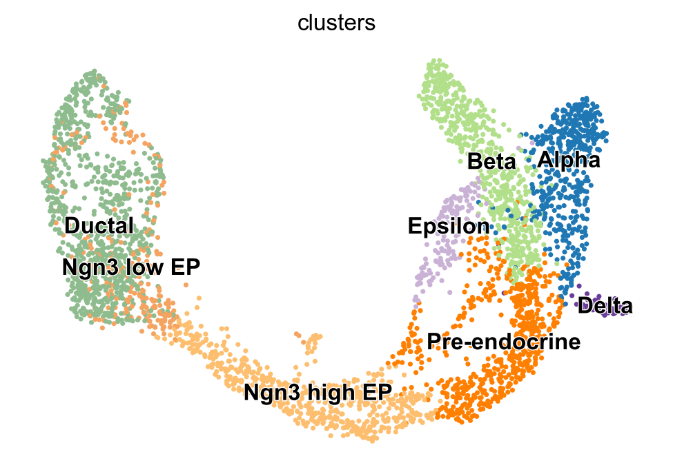

RNA velocity inference - Steady-state model¶

As a first step, we calculate RNA velocity under the steady state model. In this case, we call scVelo’s velocity function with mode="deterministic".

scv.tl.velocity(adata, mode="deterministic")

computing velocities
    finished (0:00:00) --> added 
    'velocity', velocity vectors for each individual cell (adata.layers)

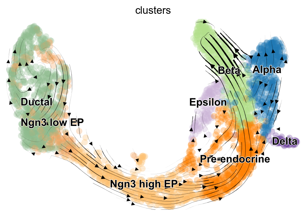
While we do not encourage over interpreting projections of high-dimensional velocity vectors onto a low dimensional representation of the data, scVelo offers a simple way of doing so.

scv.tl.velocity_graph(adata, n_jobs=8)
scv.pl.velocity_embedding_stream(adata, basis="umap", color="clusters")

computing velocity graph (using 8/8 cores)
    finished (0:00:16) --> added 
    'velocity_graph', sparse matrix with cosine correlations (adata.uns)
computing velocity embedding
    finished (0:00:00) --> added
    'velocity_umap', embedded velocity vectors (adata.obsm)

RNA velocity inference - EM model¶

In order to calculate RNA velocity with the EM model, the parameters of splicing kinetics need to be inferred first. The inference is taken care of by scVelo’s recover_dynamics function. This step might take a little while.

scv.tl.recover_dynamics(adata, n_jobs=8)

recovering dynamics (using 8/8 cores)
    finished (0:02:11) --> added 
    'fit_pars', fitted parameters for splicing dynamics (adata.var)

The parameters of the splicing model are inferred by maximizing a given likelihood. To study which genes were fit most confidently by scVelo, we can study the corresponding phase portraits as well as the inferred trajectory (plotted in purple) and steady-state ratio (dashed purple line). Here, three out of the five shown genes (Pcsk2, Top2a, Ppp1r1a) exhibit phase portraits in a (partial) almond shape. We observe a clear transition either within a single cell type (Top2a, Ppp1r1a) or across several cell types (Pcsk2, from Pre-endocrine to Alpha and Beta). In the case of Nfib, we observe two cellular populations in steady state. This is most likely an artifact of undersampling the phenotypic manifold around Ngn3 low/high EP cells. Similarly, Ghrl is highly expressed in Epsilon cells although only a few due to the small cluster size. While current best practices are limited to analysing model fits and the confidence therein by hand, recently proposed methods can help automate the process (New directions). Here, Nfib and Ghrl would be assigned with a lower confidence score.

top_genes = adata.var["fit_likelihood"].sort_values(ascending=False).index
scv.pl.scatter(adata, basis=top_genes[:5], color="clusters", frameon=False)

Having estimated the kinetics rates (stored as columns fit_alpha, fit_beta, fit_gamma of adata.obs), we can calculate both velocity and the projection onto our two-dimensional UMAP embedding.

scv.tl.velocity(adata, mode="dynamical")
scv.tl.velocity_graph(adata, n_jobs=8)
scv.pl.velocity_embedding_stream(adata, basis="umap")

computing velocities
    finished (0:00:04) --> added 
    'velocity', velocity vectors for each individual cell (adata.layers)
computing velocity graph (using 8/8 cores)
    finished (0:00:05) --> added 
    'velocity_graph', sparse matrix with cosine correlations (adata.uns)
computing velocity embedding
    finished (0:00:00) --> added
    'velocity_umap', embedded velocity vectors (adata.obsm)

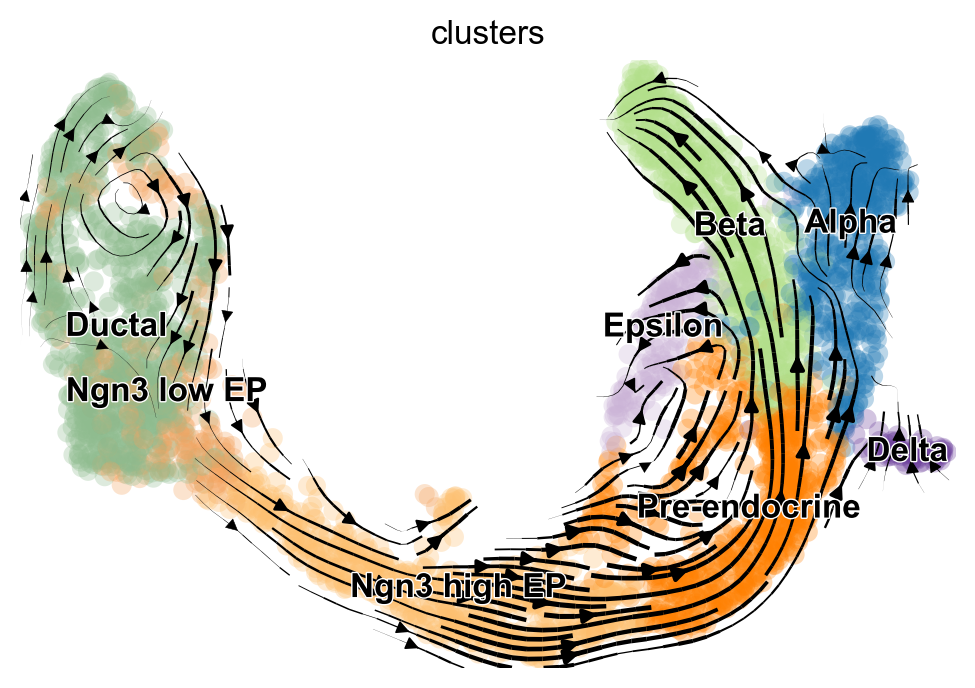
Based on the 2D projections, the EM model captures the cell cycle in the Ductal cells more faithfully. Additionally, the projection of the steady-state model exhibits a “backflow” from Alpha to Pre-endocrine cells. However, for a rigorous and quantitative analysis, we recommend using downstream tools such as CellRank Lange et al., 2022 to assess model differences and draw conclusions.

New directions¶

Although RNA velocity has been applied successfully to many systems, some model limitations persist. Violated model assumptions may cause erroneous results Bergen et al., 2021Barile et al., 2021, and projecting the high-dimensional velocity vectors onto a low-dimensional representation of the data may be misleading. To overcome these pitfalls, several tools have been developed. CellRank Lange et al., 2022, for example, uses the inferred velocity field to infer likely future states of a cell. As the algorithm operates on the higher-dimensional representation of the data, misleading velocity streams in the embeddings are avoided. Contrastingly, a recent publication tries to improve the quality of the lower-dimensional embedding Marot-Lassauzaie et al., 2022.

To soften current assumptions of RNA velocity inference, several new approaches have been suggested Qiao & Huang, 2021Marot-Lassauzaie et al., 2022Chen et al., 2022Riba et al., 2022Gu et al., 2022Gu et al., 2022, Gayoso et al., 2022. For example, these methods try to no longer assume constant rates Chen et al., 2022Gu et al., 2022, work with raw counts Gu et al., 2022, or reformulate the inference methods in a variational inference framework to associate uncertainty with estimates Gayoso et al., 2022. Additionally, to aid in understanding if RNA velocity analysis can be inferred for individual genes or entire datasets, different procedures have been proposed Zheng et al., 2022Gayoso et al., 2022.

Contributors¶

We gratefully acknowledge the contributions of:

Authors¶

Philipp Weiler
Seo H. Kim

Reviewers¶

Lukas Heumos

References¶

Manno, G. L., Soldatov, R., Zeisel, A., Braun, E., Hochgerner, H., Petukhov, V., Lidschreiber, K., Kastriti, M. E., Lönnerberg, P., Furlan, A., Fan, J., Borm, L. E., Liu, Z., van Bruggen, D., Guo, J., He, X., Barker, R., Sundström, E., Castelo-Branco, G., … Kharchenko, P. V. (2018). RNA velocity of single cells. Nature, 560(7719), 494–498. 10.1038/s41586-018-0414-6
Srivastava, A., Malik, L., Smith, T., Sudbery, I., & Patro, R. (2019). Alevin efficiently estimates accurate gene abundances from dscRNA-seq data. Genome Biology, 20(1). 10.1186/s13059-019-1670-y
He, D., Zakeri, M., Sarkar, H., Soneson, C., Srivastava, A., & Patro, R. (2022). Alevin-fry unlocks rapid, accurate and memory-frugal quantification of single-cell RNA-seq data. Nature Methods, 19(3), 316–322. 10.1038/s41592-022-01408-3
Melsted, P., Booeshaghi, A. S., Liu, L., Gao, F., Lu, L., Min, K. H., da Veiga Beltrame, E., Hjörleifsson, K. E., Gehring, J., & Pachter, L. (2021). Modular, efficient and constant-memory single-cell RNA-seq preprocessing. Nature Biotechnology, 39(7), 813–818. 10.1038/s41587-021-00870-2
Zeisel, A., Köstler, W. J., Molotski, N., Tsai, J. M., Krauthgamer, R., Jacob-Hirsch, J., Rechavi, G., Soen, Y., Jung, S., Yarden, Y., & Domany, E. (2011). Coupled pre-mRNA and mRNA dynamics unveil operational strategies underlying transcriptional responses to stimuli. Molecular Systems Biology, 7(1), 529. 10.1038/msb.2011.62
Bergen, V., Lange, M., Peidli, S., Wolf, F. A., & Theis, F. J. (2020). Generalizing RNA velocity to transient cell states through dynamical modeling. Nature Biotechnology, 38(12), 1408–1414. 10.1038/s41587-020-0591-3
Bergen, V., Soldatov, R. A., Kharchenko, P. V., & Theis, F. J. (2021). RNA velocity—current challenges and future perspectives. Molecular Systems Biology, 17(8). 10.15252/msb.202110282
Barile, M., Imaz-Rosshandler, I., Inzani, I., Ghazanfar, S., Nichols, J., Marioni, J. C., Guibentif, C., & Goettgens, B. (2021). Coordinated changes in gene expression kinetics underlie both mouse and human erythroid maturation. Genome Biology, 22(1). 10.1186/s13059-021-02414-y
Bastidas-Ponce, A., Tritschler, S., Dony, L., Scheibner, K., Tarquis-Medina, M., Salinno, C., Schirge, S., Burtscher, I., Boettcher, A., Theis, F., Lickert, H., & Bakhti, M. (2019). Massive single-cell mRNA profiling reveals a detailed roadmap for pancreatic endocrinogenesis. Development. 10.1242/dev.173849
Lange, M., Bergen, V., Klein, M., Setty, M., Reuter, B., Bakhti, M., Lickert, H., Ansari, M., Schniering, J., Schiller, H. B., Pe’er, D., & Theis, F. J. (2022). CellRank for directed single-cell fate mapping. Nature Methods, 19(2), 159–170. 10.1038/s41592-021-01346-6
Marot-Lassauzaie, V., Bouman, B. J., Donaghy, F. D., Demerdash, Y., Essers, M. A. G., & Haghverdi, L. (2022). Towards reliable quantification of cell state velocities. PLOS Computational Biology, 18(9), e1010031. 10.1371/journal.pcbi.1010031
Qiao, C., & Huang, Y. (2021). Representation learning of RNA velocity reveals robust cell transitions. Proceedings of the National Academy of Sciences, 118(49). 10.1073/pnas.2105859118
Chen, Z., King, W. C., Hwang, A., Gerstein, M., & Zhang, J. (2022). Single-cell transcriptomic deep velocity field learning with neural ordinary differential equations. Science Advances, 8(48). 10.1126/sciadv.abq3745
Riba, A., Oravecz, A., Durik, M., Jiménez, S., Alunni, V., Cerciat, M., Jung, M., Keime, C., Keyes, W. M., & Molina, N. (2022). Cell cycle gene regulation dynamics revealed by RNA velocity and deep-learning. Nature Communications, 13(1). 10.1038/s41467-022-30545-8
Gu, Y., Blaauw, D., & Welch, J. D. (2022). Bayesian Inference of RNA Velocity from Multi-Lineage Single-Cell Data. bioarXiv. 10.1101/2022.07.08.499381