Data integration

Motivation¶

A central challenge in most scRNA-seq data analyses is presented by batch effects. Batch effects are changes in measured expression levels that are the result of handling cells in distinct groups or “batches”. For example, a batch effect can arise if two labs have taken samples from the same cohort, but these samples are dissociated differently. If Lab A optimizes its dissociation protocol to dissociate cells in the sample while minimizing the stress on them, and Lab B does not, then it is likely that the cells in the data from the group B will express more stress-linked genes (JUN, JUNB, FOS, etc. see Brink et al., 2017) even if the cells had the same profile in the original tissue. In general, the origins of batch effects are diverse and difficult to pin down. Some batch effect sources might be technical, such as differences in sample handling, experimental protocols, or sequencing depths, but biological effects such as donor variation, tissue, or sampling location are also often interpreted as a batch effect Luecken et al., 2021. Whether biological factors should be considered as batch effects depends on the experimental design and the question being asked. Removing batch effects is crucial to enable joint analysis that can focus on identifying common structure in the data across batches, allowing us to perform queries across datasets. Often, it is only after removing these effects that rare cell populations can be identified that were previously obscured by differences between batches. Enabling queries across datasets allows us to ask questions that could not be answered by analysing individual datasets, such as Which cell types express SARS-CoV-2 entry factors and how does this expression differ between individuals? Muus et al., 2021.

When removing batch effects from omics data, one must make two central choices: (1) the method and parameterization, and (2) the batch covariate. As batch effects can arise between groupings of cells at different levels (i.e., samples, donors, datasets, etc.), the choice of batch covariate indicates which level of variation should be retained and which level removed. The finer the batch resolution, the more effects will be removed. However, fine batch variation is also more likely to be confounded with biologically meaningful signals. For example, samples typically come from different individuals or different locations in the tissue. These effects may be worth examining. Thus, the choice of batch covariate will depend on the goal of your integration task. Do you want to see differences between individuals, or are you focused on common variations within cell types? An approach to batch covariate selection based on quantitative analyses was pioneered in a recent effort to build an integrated atlas of the human lung, where the variance attributable to different technical covariates was used to make this choice Sikkema et al., 2022.

Types of integration models¶

Methods that remove batch effects in scRNA-seq are typically composed of (up to) three steps:

1. Dimensionality reduction

2. Modeling and removing the batch effect

3. Projection back into a high-dimensional space

While modeling and removing the batch effect (Step 2) is the central part of any batch removal method, many methods first project the data to a lower dimensional space (Step 1) to improve the signal-to-noise ratio (see the dimensionality reduction chapter) and perform batch correction in that space to achieve better performance (see Luecken et al., 2021). In the third step, a method may project the data back into the original high-dimensional feature space after removing the fitted batch effect, thereby outputting a batch-corrected gene expression matrix.

Batch-effect removal methods can vary in each of these three steps. They may use various linear or non-linear dimensionality reduction approaches, linear or non-linear batch effect models, and output different formats of batch-corrected data. Overall, we can divide methods for batch effect removal into 4 categories. In their order of development, these are global models, linear embedding models, graph-based methods, and deep learning approaches (Fig. I1).

Global models originate from bulk transcriptomics and model the batch effect as a consistent (additive and/or multiplicative) effect across all cells. A common example is ComBat Johnson et al., 2007.

Linear embedding models were the first single-cell-specific batch removal methods. These approaches often use a variant of singular value decomposition (SVD) to embed the data, then look for local neighborhoods of similar cells across batches in the embedding, which they use to correct the batch effect in a locally adaptive (non-linear) manner. Methods often project the data back into gene expression space using the SVD loadings, but may also only output a corrected embedding. This is the most common group of methods and prominent examples include the pioneering mutual nearest neighbors (MNN) method Haghverdi et al., 2018 (which does not perform any dimensionality reduction), Seurat integration Butler et al., 2018Stuart et al., 2019, Scanorama Hie et al., 2019, FastMNN Haghverdi et al., 2018, and Harmony Korsunsky et al., 2019.

Graph-based methods are typically the fastest methods to run. These approaches use a nearest-neighbor graph to represent the data from each batch. Batch effects are corrected by forcing connections between cells from different batches and then allowing for differences in cell type compositions by pruning the forced edges. The most prominent example of these approaches is the Batch-Balanced k-Nearest Neighbor (BBKNN) method Polański et al., 2019.

Deep learning (DL) approaches are the most recent, and most complex methods for batch effect removal that typically require the most data for good performance. Most deep learning integration methods are based on autoencoder networks, where either the dimensionality reduction is conditioned on the batch covariate in a conditional variational autoencoder (CVAE) or a locally linear correction is fitted in the embedded space. Prominent examples of DL methods are scVI Lopez et al., 2018, scANVI Xu et al., 2021, and scGen Lotfollahi et al., 2019.

Some methods can use cell identity labels to provide the method with a reference for what biological variation should not be removed as a batch effect. As batch-effect removal is typically a preprocessing task, such approaches may not be applicable to many integration scenarios, as labels are generally not yet available at this stage.

More detailed overviews of batch-effect removal methods can be found in Argelaguet et al., 2021 and Luecken et al., 2021.

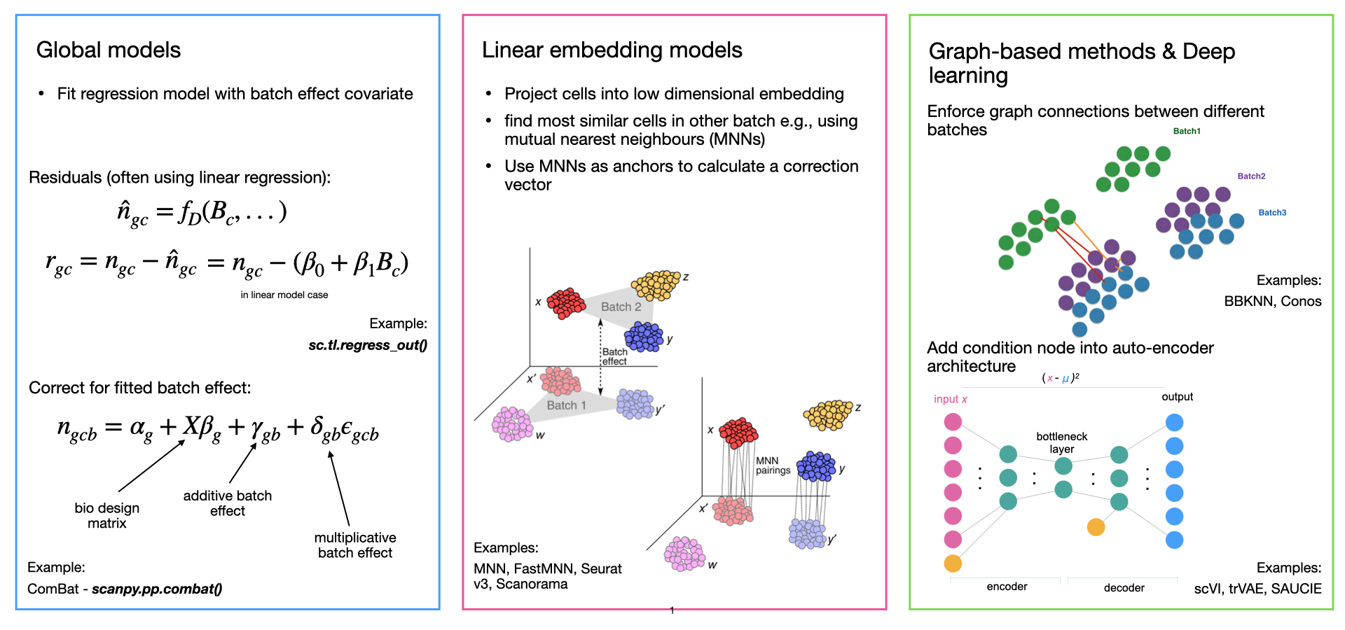Fig. I1: Overview of different types of integration methods with examples.

Batch removal complexity¶

The removal of batch effects in scRNA-seq data has previously been divided into two subtasks: batch correction and data integration Luecken & Theis, 2019. These subtasks differ in the complexity of the batch effect that must be removed. Batch correction methods address batch effects between samples in the same experiment, where cell identity compositions are consistent, and the effect is often quasi-linear. In contrast, data integration methods deal with complex, often nested, batch effects between datasets that may be generated using different protocols, where cell identities may not be shared across batches. While we use this distinction here, it is worth noting that these terms are often used interchangeably in general usage. Given the differences in complexity, it is not surprising that different methods have been benchmarked as being optimal for these two subtasks.

Comparisons of data integration methods¶

Several benchmarks have previously evaluated the performance of methods for batch correction and data integration. When removing batch effects, methods may overcorrect and remove meaningful biological variation in addition to the batch effect. For this reason, it is important that integration performance is evaluated by considering both batch effect removal and the conservation of biological variation.

The k-nearest-neighbor Batch-Effect Test (kBET) was the first metric for quantifying batch correction of scRNA-seq data Büttner et al., 2019. Using kBET, the authors found that ComBat outperformed other approaches for batch correction while comparing predominantly global models. Building on this, two recent benchmarks Tran et al., 2020 and Chazarra-Gil et al., 2021 also benchmarked linear-embedding and deep-learning models on batch correction tasks with few batches or low biological complexity. These studies found that the linear-embedding models Seurat Butler et al., 2018Stuart et al., 2019 and Harmony Korsunsky et al., 2019 performed well for simple batch correction tasks.

Benchmarking complex integration tasks poses additional challenges due to both the size and number of datasets, as well as the diversity of scenarios. Recently, a large study used 14 metrics to benchmark 16 methods across integration method classes on five RNA tasks and two simulations Luecken et al., 2021. While top-performing methods varied by task, approaches that utilized cell type labels performed better across tasks. Furthermore, deep learning approaches scANVI (with labels), scVI, and scGen (with labels), as well as the linear embedding model Scanorama, performed best, particularly on complex tasks, while Harmony performed well on less complex tasks. A similar benchmark performed for the specific purpose of integrating retina datasets to build an ocular mega-atlas also found that scVI outperformed other methods Swamy et al., 2021.

Choosing an integration method¶

While integration methods have now been extensively benchmarked, an optimal method for all scenarios does not exist. Packages of integration performance metrics and evaluation pipelines like scIB and batchbench can be used to evaluate integration performance on your own data. However, many metrics (particularly those that measure the conservation of biological variation) require ground-truth cell identity labels. Parameter optimization may tune many methods to work for particular tasks, yet in general, one can say that Harmony and Seurat consistently perform well for simple batch correction tasks, and scVI, scGen, scANVI, and Scanorama perform well for more complex data integration tasks. When choosing a method, we recommend considering these options first. Additionally, frameworks like Open Problems provide benchmarking platforms, including a leaderboard with results from various tasks such as batch integration Luecken et al., 2025.

Furthermore, the choice of integration method may be guided by the required output data format (i.e., do you need corrected gene expression data or does an integrated embedding suffice?). It would be prudent to test multiple methods and evaluate the outputs based on quantitative definitions of success before selecting one. Extensive guidelines for choosing a data integration method can be found in Luecken et al., 2021.

In the rest of this chapter, we demonstrate some of the best-performing methods and quickly demonstrate how integration performance can be evaluated.

Let’s silence some warnings, that will not affect our code:

Now setting up the environments:

Current environment dependencies are pinned to older versions of Python and Scanpy for BBKNN compatibility. A version upgrade is planned following the upcoming integration of BBKNN into the Scanpy library.

Dataset¶

The dataset we will use to demonstrate data integration contains several samples of bone marrow mononuclear cells. These samples were originally created for the Open Problems in Single-Cell Analysis NeurIPS Competition 2021 Luecken et al., 2022Lance et al., 2022. The 10x Multiome protocol was used which measures both RNA expression (scRNA-seq) and chromatin accessibility (scATAC-seq) in the same cells. The version of the data we use here was already pre-processed to remove low-quality cells.

Let’s read in the dataset using scanpy to get an AnnData object.

The full dataset contains 69,249 cells and measurements for 129,921 features. There are two versions of the expression matrix, counts, which contains the raw count values, and logcounts, which contains normalized log counts (these values are also stored in adata.X).

The obs slot contains several variables, some of which were calculated during pre-processing (for quality control) and others that contain metadata about the samples. The ones we are interested in here are:

• cell_type - The annotated label for each cell

• batch - The sequencing batch for each cell

For a real analysis, it would be important to consider more variables, but to keep it simple here, we will only look at these.

We define variables to hold these names so that it is clear how we are using them in the code. This also helps with reproducibility because if we decide to change one of them for whatever reason, we can be sure it has changed throughout the entire notebook.

Now, let’s review the batches and their cell counts.

There are 13 different batches in the dataset. During this experiment, multiple samples were taken from a set of donors and sequenced at different facilities so the names here are a combination of the sample number (eg. “s1”) and the donor (eg. “d2”). For simplicity, and to reduce computational time, we will select three samples to use.

After subsetting to select these batches we are left with 10,270 cells.

We have two annotations for the features stored in var:

• feature_types - The type of each feature (RNA or ATAC)

• gene_id - The gene associated with each feature

Let’s have a look at the feature types.

We can see that there are over 100,000 ATAC features, but only around 13,000 gene expression (“GEX”) features. Integration of multiple modalities is a complex problem that will be described in the multimodal integration chapter, so for now we will subset to only the gene expression features. We also perform simple filtering to make sure we have no features with zero counts (this is necessary because by selecting a subset of samples, we may have removed all the cells that expressed a particular feature).

Because of the subsetting we also need to re-normalise the data. Here we just normalise using global scaling by the total counts per cell.

We will use this dataset to demonstrate integration.

Most integration methods require a single object containing all the samples and a batch variable (like we have here). If instead, you have separate objects for each of your samples you can join them using the anndata concat() function. See the concatenation tutorial for more details. Similar functionality exists in other ecosystems.

Unintegrated data¶

It is always recommended to look at the raw data before performing any integration. This can provide some indication of the magnitude of any batch effects and what might be causing them (and therefore which variables to consider as the batch label). For some experiments, it might even suggest that integration is not required if samples already overlap. This is not uncommon for mouse or cell line studies from a single lab, for example, where most of the variables that contribute to batch effects can be controlled (i.e., the batch correction setting).

We will perform highly variable gene (HVG) selection, PCA, and UMAP dimensionality reduction as we have seen in previous chapters.

This adds several new items to our AnnData object. The var slot now includes means, dispersions and the selected variable genes. In the obsp slot we have distances and connectivities for our KNN graph and in obsm are the PCA and UMAP embeddings.

Let’s plot the UMAP, colouring the points by cell identity and batch labels. If the dataset had not already been labelled (which is often the case) we would only be able to consider the batch labels.

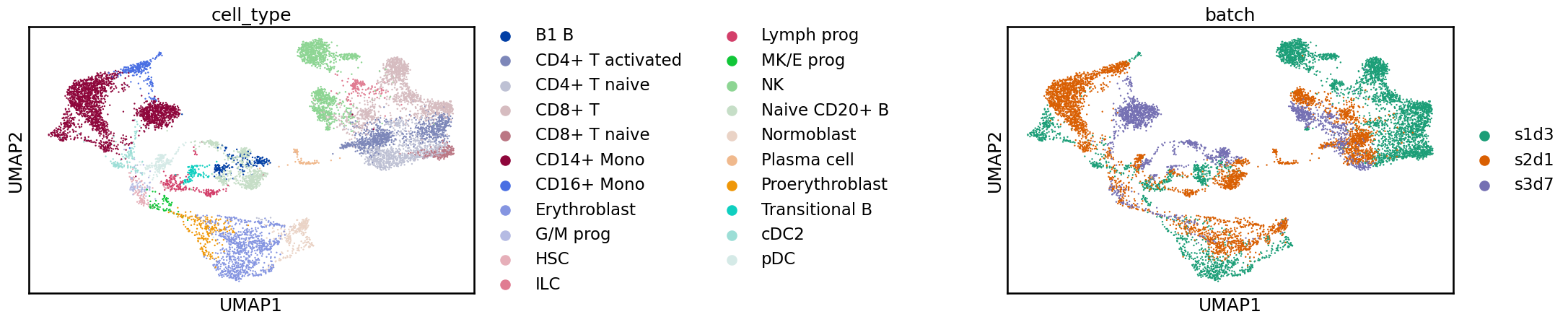
Often, when examining these plots, you will notice a clear separation between batches. In this case, what we see is more subtle, and while cells from the same label are generally near each other, there is a shift between batches. If we were to perform a clustering analysis using this raw data, we would probably end up with some clusters containing a single batch, which would be difficult to interpret at the annotation stage. We are also likely to overlook rare cell types that are not common enough in any single sample to produce their own cluster. While UMAPs can often display batch effects, it is always important, when considering these 2D representations, not to overinterpret them. For a real analysis, you should confirm the integration in other ways, such as by inspecting the distribution of marker genes. In the “Benchmarking your own integration” section below, we discuss metrics for quantifying the quality of an integration.

Now that we have confirmed the presence of batch effects that need to be corrected, we can proceed to the various integration methods. If the batches perfectly overlaid each other, or we could discover meaningful cell clusters without correction, then there would be no need to perform integration.

Batch-aware feature selection¶

As shown in previous chapters, we often select a subset of genes to use for our analysis in order to reduce noise and processing time. We follow the same approach when we have multiple samples; however, it is crucial that gene selection is performed in a batch-aware manner. This is because genes that are variable across the whole dataset could be capturing batch effects rather than the biological signals we are interested in. It also helps to select genes relevant to rare cell identities.

For example, if an identity is only present in one sample, then markers for it may not be variable across all samples, but should be present in that one sample.

We can perform batch-aware highly variable gene selection by setting the batch_key argument in the scanpy highly_variable_genes() function. scanpy will then calculate HVGs for each batch separately and combine the results by selecting those genes that are highly variable in the highest number of batches. We use the scanpy function here because it has built-in batch awareness. For other methods, we would have to run them on each batch individually and then manually combine the results.

We can see there are now some additional columns in var:

• highly_variable_nbatches - The number of batches where each gene was found to be highly variable

• highly_variable_intersection - Whether each gene was highly variable in every batch

• highly_variable - Whether each gene was selected as highly variable after combining the results from each batch

Let’s check how many batches each gene was variable in:

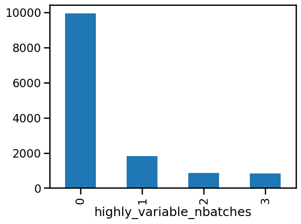
The first thing we notice is that most genes are not highly variable. This is typically the case, but it can depend on how different the samples we are trying to integrate are. The overlap then decreases as we add more samples, with relatively few genes being highly variable in all three batches. By selecting the top 2000 genes, we have selected all HVGs that are present in two or three batches and most of those that are present in one batch.

We will create an object with just the selected genes to use for integration.

Variational autoencoder (VAE) based integration¶

The first integration method we will use is scVI (single-cell Variational Inference), a method based on a conditional variational autoencoder Lopez et al., 2018 available in the scvi-tools package Gayoso et al., 2022. A variational autoencoder is a type of artificial neural network that attempts to reduce the dimensionality of a dataset. The conditional part refers to conditioning this dimensionality reduction process on a particular covariate (in this case, batches) such that the covariate does not affect the low-dimensional representation. In benchmarking studies scVI has been shown to perform well across a range of datasets with a good balance of batch correction while conserving biological variability Luecken et al., 2021. scVI models raw counts directly, so it is important that we provide it with a count matrix rather than a normalized expression matrix.

First, let’s make a copy of our dataset to use for this integration. Normally, it is not necessary to do this, but as we will demonstrate multiple integration methods, making a copy makes it easier to show what has been added by each method.

Data preparation¶

The first step in using scVI is to prepare our AnnData object. This step stores some information required by scVI such as which expression matrix to use and what the batch key is.

The fields created by scVI are prefixed with _scvi. These are designed for internal use and should not be manually modified. The general advice from the scvi-tools authors is not to make any changes to our object until after the model is trained. On other datasets, you may see a warning about the input expression matrix containing unnormalised count data. This usually means you should check that the layer provided to the setup function does actually contain count values but it can also happen if you have values from performing gene length correction on data from a full-length protocol or from another quantification method that does not produce integer counts.

Building the model¶

We can now construct an scVI model object. As well as the scVI model we use here, the scvi-tools package contains various other models (we will use the scANVI model below).

The scVI model object contains the provided AnnData object as well as the neural network for the model itself. You can see that currently the model is not trained. If we wanted to modify the structure of the network, we could provide additional arguments to the model construction function, but here we just use the defaults.

We can also print a more detailed description of the model that shows us where things are stored in the associated AnnData object.

Here we can see exactly what information has been assigned by scVI, including details like how each different batch is encoded in the model.

Training the model¶

The model will be trained for a given number of epochs, a training iteration where every cell is passed through the network. By default scVI uses the following heuristic to set the number of epochs. For datasets with fewer than 20,000 cells, 400 epochs will be used, and as the number of cells grows above 20,000, the number of epochs is continuously reduced. The reasoning behind this is that as the network sees more cells during each epoch, it can learn the same amount of information as it would from more epochs with fewer cells.

We now train the model for the selected number of epochs (this will take ~20-40 minutes depending on the computer you are using).

Extracting the embedding¶

The main result we want to extract from the trained model is the latent representation for each cell. This is a multi-dimensional embedding where the batch effects have been removed, which can be used in a similar way to how we use PCA dimensions when analysing a single dataset. We store this in obsm with the key X_scvi.

Calculate a batch-corrected UMAP¶

We will now visualise the data as we did before integration. We calculate a new UMAP embedding but instead of finding nearest neighbors in PCA space, we start with the corrected representation from scVI.

Once we have the new UMAP representation we can plot it colored by batch and identity labels as before.

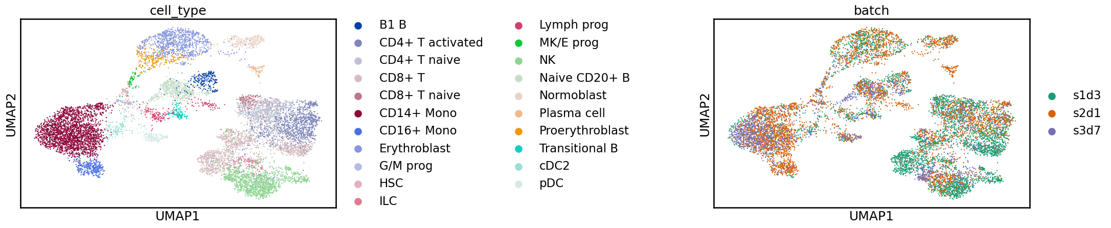
This looks better! Before, the various batches were shifted apart from each other. Now, the batches overlap more, and we have a single blob for each cell identity label.

In many cases, we would not already have identity labels, so from this stage, we would continue with clustering, annotation, and further analysis as described in other chapters.

VAE integration using cell labels¶

When performing integration with scVI we pretended that we didn’t already have any cell labels (although we showed them in plots). While this scenario is common, there are some cases where we do know something about cell identity in advance. Most often, this is when we want to combine one or more publicly available datasets with data from a new study. When we have labels for at least some of the cells we can use scANVI (single-cell ANnotation using Variational Inference) Xu et al., 2021. This is an extension of the scVI model that can incorporate cell identity label information as well as batch information. Because it has this extra information, it can try to keep the differences between cell labels while removing batch effects. Benchmarking suggests that scANVI tends to better preserve biological signals compared to scVI but sometimes it is not as effective at removing batch effects Luecken et al., 2021. While we have labels for all cells here it is also possible to use scANVI in a semi-supervised manner where labels are only provided for some cells.

We start by creating a scANVI model object. Note that because scANVI refines an already trained scVI model, we provide the scVI model rather than an AnnData object. If we had not already trained an scVI model we would need to do that first. We also provide a key for the column of adata.obs which contains our cell labels as well as the label which corresponds to unlabelled cells. In this case, all of our cells are labelled, so we just provide a dummy value. In most cases, it is important to check that this is set correctly so that scANVI knows which label to ignore during training.

This scANVI model object is very similar to what we saw before for scVI. As mentioned previously, we could modify the structure of the model network but here we just use the default parameters.

Again, we have a heuristic for selecting the number of training epochs. Note that this is much fewer than before as we are just refining the scVI model, rather than training a whole network from scratch.

We can extract the new latent representation from the model and create a new UMAP embedding as we did for scVI.

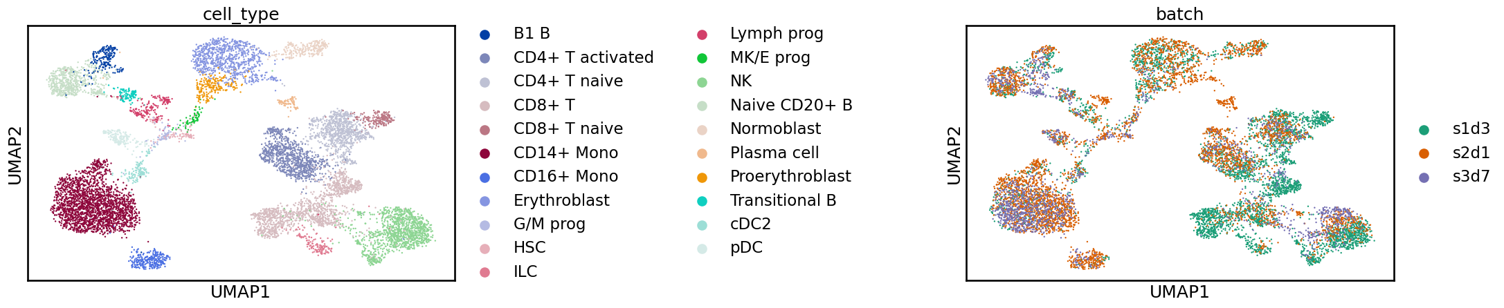
By looking at the UMAP representation it is difficult to tell the difference between scANVI and scVI but as we will see below there are differences in metric scores when the quality of the integrations is quantified. This is a reminder that we shouldn’t overinterpret these two-dimensional representations, especially when comparing methods.

Graph-based integration¶

The next method we will look at is BBKNN or “Batch Balanced KNN” Polański et al., 2019. This is a very different approach to scVI, which rather than using a neural network to embed cells in a batch corrected space, instead modifies how the k-nearest neighbor (KNN) graph used for clustering and embedding is constructed. As we have seen in previous chapters, the normal KNN procedure connects cells to the most similar cells across the whole dataset. The change that BBKNN makes is to enforce that cells are connected to cells from other batches. While this is a simple modification, it can be quite effective, particularly when there are very strong batch effects. However, as the output is an integrated graph, it can have limited downstream uses, as few packages will accept this as an input.

An important parameter for BBKNN is the number of neighbors per batch. A suggested heuristic for this is to use 25 if there are more than 100,000 cells or the default of 3 if there are fewer than 100,000.

Before using BBKNN we first perform a PCA as we would before building a normal KNN graph. Unlike scVI which models raw counts here, we start with the log-normalised expression matrix.

We can now run BBKNN, replacing the call to the scanpy neighbors() function in a standard workflow. An important difference is to make sure the batch_key argument is set which specifies a column in adata_hvg.obs that contains batch labels.

Unlike the default scanpy function, BBKNN does not allow specifying a key for storing results so they are always stored under the default “neighbors” key.

We can use this new integrated graph just like we would use a normal KNN graph to construct a UMAP embedding.

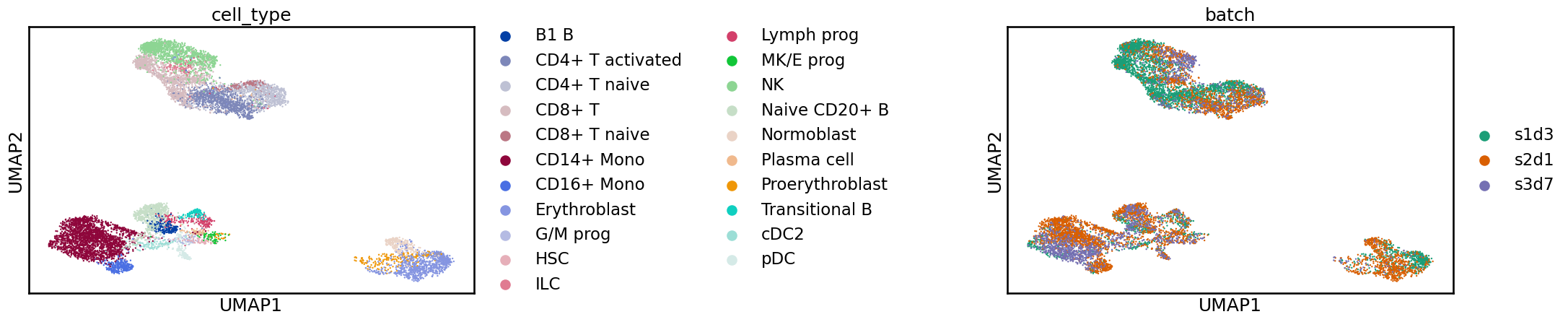
This integration is also improved compared to the unintegrated data, with cell identities grouped together, but we still see some shifts between batches.

Linear embedding integration using Mutual Nearest Neighbors (MNN)¶

Some downstream applications cannot accept an integrated embedding or neighborhood graph and require a corrected expression matrix. One approach that can produce this output is the integration method in Seurat Satija et al., 2015Butler et al., 2018Stuart et al., 2019. The Seurat integration method belongs to a class of linear embedding models that make use of the idea of mutual nearest neighbors (which Seurat calls anchors) to correct batch effects Haghverdi et al., 2018. Mutual nearest neighbors are pairs of cells from two different datasets that are in the neighborhood of each other when the datasets are placed in the same (latent) space. After finding these cells, they can be used to align the two datasets and correct the differences between them. Seurat has also been found to be one of the top mixing methods in some evaluations Tran et al., 2020.

As Seurat is an R package we must transfer our data from Python to R. Here we prepare the AnnData to convert so that it can be handled by rpy2 and anndata2ri.

The prepared AnnData is now available in R as a SingleCellExperiment object thanks to anndata2ri. Note that this is transposed compared to an AnnData object so our observations (cells) are now the columns and our variables (genes) are now the rows.

Seurat uses its own object to store data. Helpfully the authors provide a function to convert from SingleCellExperiment. We just provide the SingleCellExperiment object and tell Seurat which assays (layers in our AnnData object) contain raw counts and normalised expression (which Seurat stores in a slot called “data”).

Unlike some of the other methods, we have seen which take a single object and a batch key, the Seurat integration functions require a list of objects. We create this using the SplitObject() function.

We can now use this list to find anchors for each pair of datasets. Usually, you would identify batch-aware highly variable genes first (using the FindVariableFeatures() and SelectIntegrationFeatures() functions) but as we have done that already we tell Seurat to use all the features in the object.

Seurat can then use the anchors to compute a transformation that maps one dataset onto another. This is done in a pairwise way until all the datasets are merged. By default Seurat will determine a merge order so that more similar datasets are merged together first but it is also possible to define this order.

The result is another Seurat object, but notice now that the active assay is called “integrated”. This contains the corrected expression matrix which is the final output of the integration.

Here we extract that matrix and prepare it for transfer back to Python.

We will now store the corrected expression matrix as a layer in our AnnData object. We also set adata.X to use this matrix.

Now that we have the results of our integration we can calculate a UMAP and plot it as we have for the other methods (we could also have done this in R).

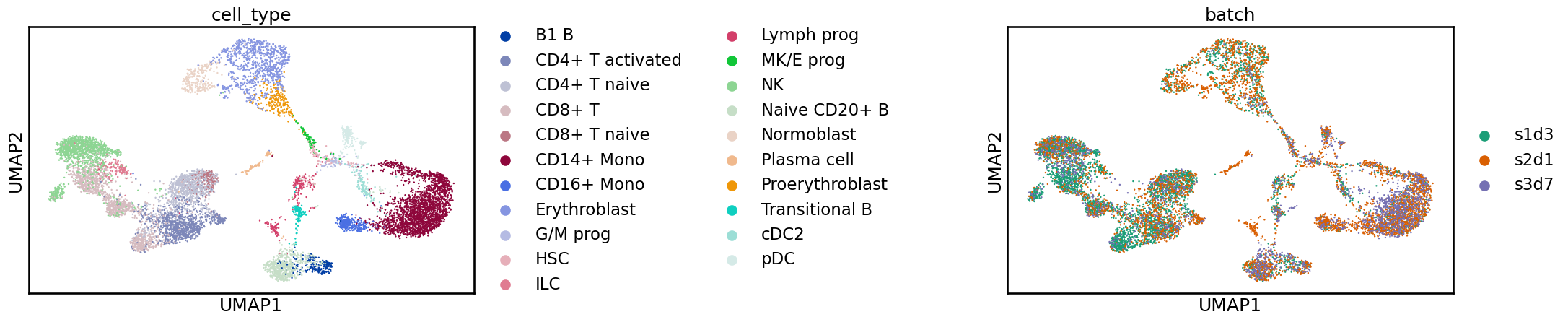
As we have previously seen, the batches are mixed while the labels are separated. It is tempting to select an integration based on the UMAPs, but this does not fully represent the quality of an integration. In the next section, we present some approaches to more rigorously evaluate integration methods.

Benchmarking your own integration¶

The methods demonstrated here are selected based on results from benchmarking experiments, including the single-cell integration benchmarking project Luecken et al., 2021. This project also produced a software package called scib that can be used to run a range of integration methods as well as the metrics that were used for evaluation. In this section, we demonstrate how to utilize this package to assess the quality of an integration.

The scib metrics can be run individually but there are also wrappers for running multiple metrics at once. Here we run a subset of the metrics, which are quick to compute using the metrics_fast() function. This function takes a few arguments: the original unintegrated dataset, the integrated dataset, a batch key, and a label key. Depending on the output of the integration method we might also need to supply additional arguments, for example here we specify the embedding to use for scVI and scANVI with the embed argument. You can also control how some metrics are run with additional arguments. Also note that you may need to check that objects are formatted properly so that scIB can find the required information.

Let’s run the metrics for each of the integrations we have performed above, as well as the unintegrated data (after highly variable gene selection).

Here is an example of what one of the metrics results looks like for a single integration:

Each row is a different metric, and the values show the score for that metric. Scores are between 0 and 1, where 1 is a good performance and 0 is a poor performance (scib can also return unscaled scores for some metrics if required). Because we have only run the fast metrics here, some of the metrics have NaN scores. Also, note that some metrics cannot be used with some output formats, which can also be a reason for NaN values being returned.

To compare the methods, it is useful to have all the metric results in one table. This code combines them and tidies them into a more convenient format.

We now have all the scores in one table with metrics as columns and methods as rows. Styling the table with a gradient can make it easier to see the differences between scores.

For some metrics, the scores tend to be in a relatively small range. To emphasise the differences between methods and place each metric on the same scale, we scale them so that the worst performer gets a score of 0, the best performer gets a score of 1 and the others are somewhere in between.

The values now better represent the differences between methods (and better match the colour scale). However, it is important to note that the scaled scores can only be used to compare the relative performance of this specific set of integrations. If we wanted to add another method, we would need to perform the scaling again. We also can’t say that an integration is definitely “good”, only that it is better than the other methods we have tried. This scaling emphasises differences between methods. For example, if we had metric scores of 0.92, 0.94, and 0.96, these would be scaled to 0, 0.5, and 1.0. This makes the first method appear to score much worse, even though it is only slightly lower than the other two and still got a very high score. This effect is bigger when comparing a few methods and when they get similar raw scores. Whether you look at raw or scaled scores depends on whether you want to focus on absolute performance or the difference in performance between methods.

The evaluation metrics can be grouped into two categories: those that measure the removal of batch effects and those that measure the conservation of biological variation. We can calculate summary scores for each of these categories by taking the mean of the scaled values for each group. This type of summary score wouldn’t make sense with raw values, as some metrics consistently produce higher scores than others (and therefore have a greater impact on the mean).

Plotting the two summary scores against each other gives an indication of the priorities of each method. Some will be biased towards batch correction while others will favour retaining biological variation.

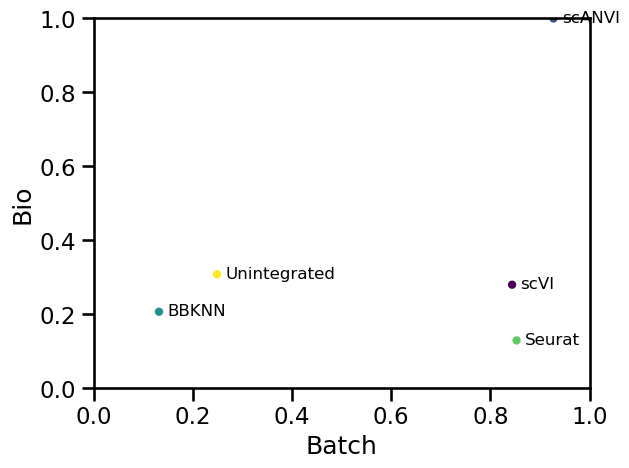
In our small example scenario BBKNN is clearly the worst performer, getting the lowest scores for both batch removal and biological conservation. The other three methods have similar batch correction scores with scANVI scoring highest for biological conservation followed by Seurat and scVI.

To get an overall score for each method, we can combine the two summary scores. The scIB paper suggests a weighting of 40% batch correction and 60% biological conservation but you may prefer to weight things differently depending on the priorities for your dataset.

Let’s make a quick bar chart to visualise the overall performance.

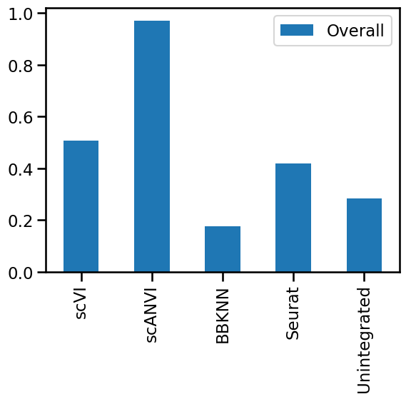
As we have already seen scANVI is the best performer followed by scVI and Seurat. It is important to note that this is just an example of how to run these metrics for this specific dataset, not a proper evaluation of these methods. For that, you should refer to existing benchmarking publications. In particular, we have only run a small selection of high-performing methods and a subset of metrics. Also, remember that scores are relative to the methods used, so even if the methods perform almost equally well, small differences will be exaggerated.

Existing benchmarks have suggested methods that generally perform well, but performance can also be quite variable across scenarios. For some analyses, it may be worthwhile performing your own evaluation of integration. The scib package makes this process easier, but it can still be a significant undertaking, relying on a good knowledge of the ground truth and interpretation of the metrics.

Quiz¶

Session information¶

Python¶

R¶

Contributors¶

We gratefully acknowledge the contributions of:

Authors¶

• Luke Zappia

• Malte Lücken

• Seo H. Kim

Reviewers¶

• Lukas Heumos